4.3 ETS taxonomy
Based on the type of error, trend and seasonality, (Pegels 1969) proposed a taxonomy, which was then developed further by (Hyndman et al. 2002) and refined by (Hyndman et al. 2008). According to this taxonomy, error, trend and seasonality can be:
- Error: either “Additive” (A), or “Multiplicative” (M);
- Trend: either “None” (N), or “Additive” (A), or “Additive damped” (Ad), or “Multiplicative” (M), or “Multiplicative damped” (Md);
- Seasonality: either “None” (N), or “Additive” (A), or “Multiplicative” (M).
So, the ETS stands for “Error-Trend-Seasonality” and defines how specifically the components interact with each other. According to this taxonomy, the model (4.1) is ETS(A,A,A), while the model (4.2) is ETS(M,M,M), and (4.3) is ETS(M,A,M).
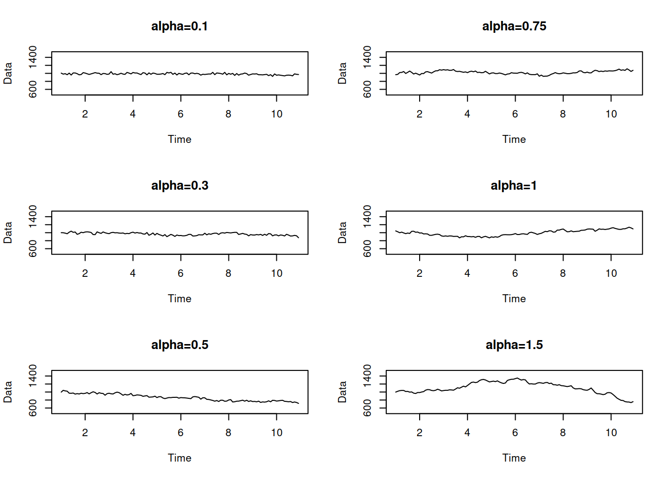
The main advantage of ETS taxonomy is that the components have clear interpretation, and that it is flexible, allowing to have 30 models with different types of error, trend and seasonality. The figure below shows examples of different time series with deterministic (they do not change over time) level, trend and seasonality, based on how they interact in the model. The first one shows the additive error case:
Things to note from this plot:
- When the seasonality is multiplicative, its amplitude increases with the increase of the level of the data. The amplitude of seasonality does not change for the additive seasonal models. e.g. compare the ETS(A,A,A) with ETS(A,A,M): the distance between the highest and the lowest points for the former in the first year is roughly the same as in the last year. In the case of ETS(A,A,M), the distance increases with the increase of level;
- When the trend is multiplicative, it corresponds to the exponential growh / decay. So, in this situation with ETS(A,M,N) we say that there is a roughly 5% growth in the data;
- The damped trend models slow down both additive and multiplicative trends;
- It is practically impossible to distinguish the additive and multiplicative seasonality if the average of the data is the same - this becomes apparent on the example of ETS(A,N,A) and ETS(A,N,M).
And here is a similar plot for the multiplicative error models:
They show roughly the same picture as the additive case, with the main difference being that the variance of the error increases with the increase of the average value of the data - this becomes clearer on ETS(M,A,N) and ETS(M,M,N) data. This effect is called heteroscedasticity in statistics, and (Hyndman et al. 2008) argue that the main benefit of the multiplicative error models is in being able to capture this feature.
In the next several chapters we will discuss the basic ETS models from this taxonomy. Note that not all the models in this taxonomy make sense, and some of them are typically dropped from consideration. Although ADAM implements all o fhtme, we will discuss the potential issues with them and what to expect from them.
References
Hyndman, Rob J., Anne B. Koehler, J. Keith Ord, and Ralph D. Snyder. 2008. Forecasting with Exponential Smoothing. Springer Berlin Heidelberg.
Hyndman, Rob J, Anne B Koehler, Ralph D Snyder, and Simone Grose. 2002. “A state space framework for automatic forecasting using exponential smoothing methods.” International Journal of Forecasting 18 (3): 439–54. https://doi.org/10.1016/S0169-2070(01)00110-8.
Pegels, C Carl. 1969. “Exponential Forecasting : Some New Variations.” Management Science 15 (5): 311–15. https://www.jstor.org/stable/2628137.