2.7 Theory of distributions
There are several probability distributions that will be helpful in the further chapters of this textbook. Here, I want to briefly discuss those of them that will be used. While this might not seem important at this point, we will refer to this section of the textbook in the next chapters.
2.7.1 Normal distribution
Every statistical textbook has Normal distribution. It is that one famous bell-curved distribution that every statistician likes because it is easy to work with and it is an asymptotic distribution for many other well-behaved distributions in some conditions (see discussion of “Central Limit Theorem” in Section 2.2.2). Here is the probability density function (PDF) of this distribution: \[\begin{equation} f(y_t) = \frac{1}{\sqrt{2 \pi \sigma^2}} \exp \left( -\frac{\left(y_t - \mu_{y,t} \right)^2}{2 \sigma^2} \right) , \tag{2.16} \end{equation}\] where \(y_t\) is the value of the response variable, \(\mu_{y,t}=\mu_{y,t|t-1}\) is the one step ahead conditional expectation on observation \(t\), given the information on \(t-1\) and \(\sigma^2\) is the variance of the error term. The maximum likelihood estimate of \(\sigma^2\) is: \[\begin{equation} \hat{\sigma}^2 = \frac{1}{T} \sum_{t=1}^T \left(y_t - \hat{\mu}_{y,t} \right)^2 , \tag{2.17} \end{equation}\] where \(T\) is the sample size and \(\hat{\mu}_{y,t}\) is the estimate of the conditional expecatation \(\mu_{y,t}\). (2.17) coincides with Mean Squared Error (MSE), discussed in the section 1.
And here how this distribution looks (Figure 2.32).
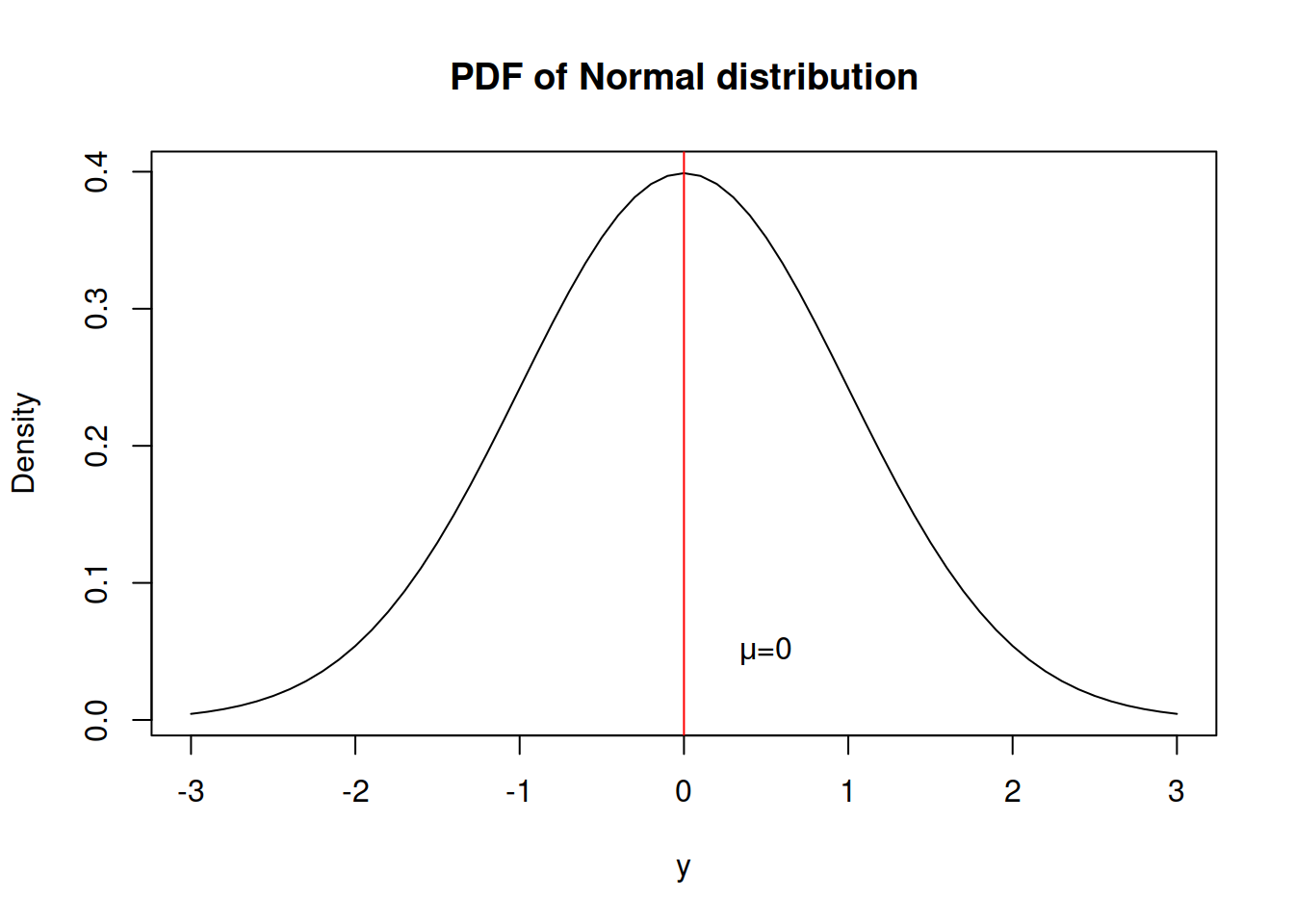
Figure 2.32: Probability Density Function of Normal distribution
What we typically assume in the basic time series models is that a variable is random and follows Normal distribution, meaning that there is a central tendency (in our case - the mean \(mu\)), around which the density of values is the highest and there are other potential cases, but their probability of appearance reduces proportionally to the distance from the centre.
The Normal distribution has skewness of zero and kurtosis of 3 (and excess kurtosis, being kurtosis minus three, of 0).
Additionally, if Normal distribution is used for the maximum likelihood estimation of a model, it gives the same parameters as the minimisation of MSE would give.
The log-likelihood based on the Normal distribution is derived by taking the sum of logarithms of the PDF of Normal distribution (2.16):
\[\begin{equation}
\ell(\mathbf{Y}| \theta, \sigma^2) = - \frac{T}{2} \log \left(2 \pi \sigma^2\right) - \sum_{t=1}^T \frac{\left(y_t - \mu_{y,t} \right)^2}{2 \sigma^2} ,
\tag{2.18}
\end{equation}\]
where \(\theta\) is the vector of all the estimated parameters in the model, and \(\log\) is the natural logarithm. If one takes the derivative of (2.18) with respect to \(\sigma^2\), then the formula (2.17) is obtained. Another useful thing to note is the concentrated log-likelihood, which is obtained by inserting the estimated variance (2.17) in (2.18):
\[\begin{equation}
\ell(\mathbf{Y}| \theta, \hat{\sigma}^2) = - \frac{T}{2} \log \left( 2 \pi e \hat{\sigma}^2 \right) ,
\tag{2.19}
\end{equation}\]
where \(e\) is the Euler’s constant. The concentrated log-likelihood is handy, when estimating the model and calculating information criteria. Sometimes, statisticians drop the \(2 \pi e\) part from the (2.19), because it does not affect any inferences, as long as one works only with Normal distribution (for example, this is what is done in ets() function from forecast package in R). However, it is not recommended to do (Burnham and Anderson, 2004), because this makes the comparison with other distributions impossible.
Normal distribution is available in stats package with dnorm(), qnorm(), pnorm() and rnorm() functions.
2.7.2 Laplace distribution
A more exotic distribution is Laplace, which has some similarities with Normal, but has higher excess. It has the following PDF:
\[\begin{equation} f(y_t) = \frac{1}{2 s} \exp \left( -\frac{\left| y_t - \mu_{y,t} \right|}{s} \right) , \tag{2.20} \end{equation}\] where \(s\) is the scale parameter, which, when estimated using likelihood, is equal to the Mean Absolute Error (MAE): \[\begin{equation} \hat{s} = \frac{1}{T} \sum_{t=1}^T \left| y_t - \hat{\mu}_{y,t} \right| . \tag{2.21} \end{equation}\]
It has the shape shown on Figure 2.33.
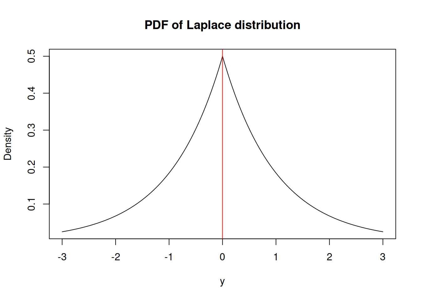
Figure 2.33: Probability Density Function of Laplace distribution
Similar to the Normal distribution, the skewness of Laplace is equal to zero. However, it has fatter tails - its kurtosis is equal to 6 instead of 3.
The variance of the random variable following Laplace distribution is equal to: \[\begin{equation} \sigma^2 = 2 s^2. \tag{2.22} \end{equation}\]
The dlaplace, qlaplace, plaplace and rlaplace functions from greybox package implement different sides of Laplace distribution in R.
2.7.3 S distribution
This is something relatively new, but not ground braking. I have derived S distribution few years ago, but have never written a paper on that. It has the following density function (it is as a special case of Generalised Normal distribution, when \(\beta=0.5\)): \[\begin{equation} f(y_t) = \frac{1}{4 s^2} \exp \left( -\frac{\sqrt{|y_t - \mu_{y,t}|}}{s} \right) , \tag{2.23} \end{equation}\] where \(s\) is the scale parameter. If estimated via maximum likelihood, the scale parameter is equal to: \[\begin{equation} \hat{s} = \frac{1}{2T} \sum_{t=1}^T \sqrt{\left| y_t - \hat{\mu}_{y,t} \right|} , \tag{2.24} \end{equation}\] which corresponds to the minimisation of a half of “Mean Root Absolute Error” or “Half Absolute Moment” (HAM). This is a more exotic type of scale, but the main benefit of this distribution is sever heavy tails - it has kurtosis of 25.2. It might be useful in cases of randomly occurring incidents and extreme values (Black Swans?).
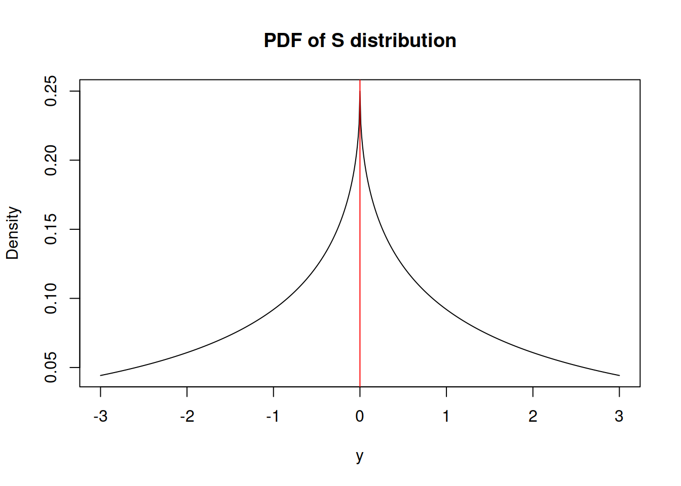
Figure 2.34: Probability Density Function of S distribution
The variance of the random variable following S distribution is equal to: \[\begin{equation} \sigma^2 = 120 s^4. \tag{2.25} \end{equation}\]
The ds, qs, ps and rs from greybox package implement the density, quantile, cumulative and random generation functions.
2.7.4 Generalised Normal distribution
Generalised Normal (\(\mathcal{GN}\)) distribution (as the name says) is a generalisation for Normal distribution, which also includes Laplace and S as special cases (Nadarajah, 2005). There are two versions of this distribution: one with a shape and another with a skewness parameter. We are mainly interested in the first one, which has the following PDF: \[\begin{equation} f(y_t) = \frac{\beta}{2 s \Gamma(\beta^{-1})} \exp \left( -\left(\frac{|y_t - \mu_{y,t}|}{s}\right)^{\beta} \right), \tag{2.26} \end{equation}\] where \(\beta\) is the shape parameter, and \(s\) is the scale of the distribution, which, when estimated via MLE, is equal to: \[\begin{equation} \hat{s} = \sqrt[^{\beta}]{\frac{\beta}{T} \sum_{t=1}^T\left| y_t - \hat{\mu}_{y,t} \right|^{\beta}}, \tag{2.27} \end{equation}\] which has MSE, MAE and HAM as special cases, when \(\beta\) is equal to 2, 1 and 0.5 respectively. The parameter \(\beta\) influences the kurtosis directly, it can be calculated for each special case as \(\frac{\Gamma(5/\beta)\Gamma(1/\beta)}{\Gamma(3/\beta)^2}\). The higher \(\beta\) is, the lower the kurtosis is.
The advantage of \(\mathcal{GN}\) distribution is its flexibility. In theory, it is possible to model extremely rare events with this distribution, if the shape parameter \(\beta\) is fractional and close to zero. Alternatively, when \(\beta \rightarrow \infty\), the distribution converges point-wise to the uniform distribution on \((\mu_{y,t} - s, \mu_{y,t} + s)\).
Note that the estimation of \(\beta\) is a difficult task, especially, when it is less than 2 - the MLE of it looses properties of consistency and asymptotic normality.
Depending on the value of \(\beta\), the distribution can have different shapes shown in Figure 2.35
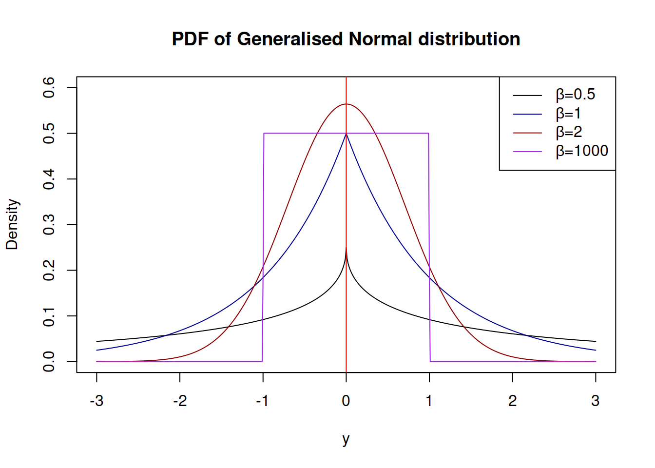
Figure 2.35: Probability Density Functions of Generalised Normal distribution
Typically, estimating \(\beta\) consistently is a tricky thing to do, especially if it is less than one. Still, it is possible to do that by maximising the likelihood function (2.26).
The variance of the random variable following Generalised Normal distribution is equal to: \[\begin{equation} \sigma^2 = s^2\frac{\Gamma(3/\beta)}{\Gamma(1/\beta)}. \tag{2.28} \end{equation}\]
The working functions for the Generalised Normal distribution are implemented in the greybox package for R.
2.7.5 Asymmetric Laplace distribution
Asymmetric Laplace distribution (\(\mathcal{AL}\)) can be considered as a two Laplace distributions with different parameters \(s\) for left and right sides from the location \(\mu_{y,t}\). There are several ways to summarise the probability density function, the neater one relies on the asymmetry parameter \(\alpha\) (Yu and Zhang, 2005): \[\begin{equation} f(y_t) = \frac{\alpha (1- \alpha)}{s} \exp \left( -\frac{y_t - \mu_{y,t}}{s} (\alpha - I(y_t \leq \mu_{y,t})) \right) , \tag{2.29} \end{equation}\] where \(s\) is the scale parameter, \(\alpha\) is the skewness parameter and \(I(y_t \leq \mu_{y,t})\) is the indicator function, which is equal to one, when the condition is satisfied and to zero otherwise. The scale parameter \(s\) estimated using likelihood is equal to the quantile loss: \[\begin{equation} \hat{s} = \frac{1}{T} \sum_{t=1}^T \left(y_t - \hat{\mu}_{y,t} \right)(\alpha - I(y_t \leq \hat{\mu}_{y,t})) . \tag{2.30} \end{equation}\] Thus maximising the likelihood (2.29) is equivalent to estimating the model via the minimisation of \(\alpha\) quantile, making this equivalent to quantile regression approach. So quantile regression models assume indirectly that the error term in the model is \(\epsilon_t \sim \mathcal{AL}(0, s, \alpha)\) (Geraci and Bottai, 2007).
Depending on the value of \(\alpha\), the distribution can have different shapes, shown in Figure 2.36.
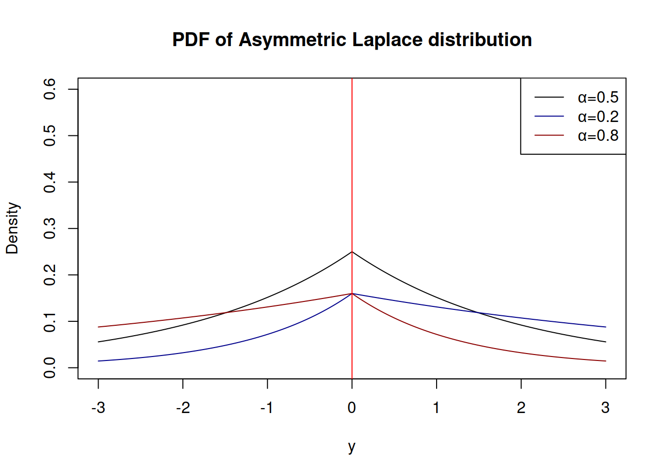
Figure 2.36: Probability Density Functions of Asymmetric Laplace distribution
Similarly to \(\mathcal{GN}\) distribution, the parameter \(\alpha\) can be estimated during the maximisation of the likelihood, although it makes more sense to set it to some specific values in order to obtain the desired quantile of distribution.
The variance of the random variable following Asymmetric Laplace distribution is equal to: \[\begin{equation} \sigma^2 = s^2\frac{(1-\alpha)^2+\alpha^2}{\alpha^2(1-\alpha)^2}. \tag{2.31} \end{equation}\]
Functions dalaplace, qalaplace, palaplace and ralaplace from greybox package implement the Asymmetric Laplace distribution.
2.7.6 Log Normal, Log Laplace, Log S and Log GN distributions
In addition, it is possible to derive the log-versions of the Normal, \(\mathcal{Laplace}\), \(\mathcal{S}\), and \(\mathcal{GN}\) distributions. The main differences between the original and the log-versions of density functions for these distributions can be summarised as follows: \[\begin{equation} f_{log}(\log(y_t)) = \frac{1}{y_t} f(\log y_t). \tag{2.32} \end{equation}\] They are defined for positive values only and will have different right tail, depending on the location, scale and shape parameters. \(\exp(\mu_{\log y,t})\) in this case represents the geometric mean (and median) of distribution rather than the arithmetic one. The conditional expectation in these distributions is typically higher than \(\exp(\mu_{\log y,t})\) and depends on the value of the scale parameter. It is known for log\(\mathcal{N}\) and is equal to: \[\begin{equation} \mathrm{E}(y_t) = \mathrm{exp}\left(\mu_{\log y,t} + \frac{\sigma^2}{2} \right). \tag{2.33} \end{equation}\] However, it does not have a simple form for the other distributions.
2.7.7 Inverse Gaussian distribution
An exotic distribution that will be useful for what comes in this textbook is the Inverse Gaussian (\(\mathcal{IG}\)), which is parameterised using mean value \(\mu_{y,t}\) and either the dispersion parameter \(s\) or the scale \(\lambda\) and is defined for positive values only. This distribution is useful because it is scalable and has some similarities with the Normal one. In our case, the important property is the following: \[\begin{equation} \text{if } (1+\epsilon_t) \sim \mathcal{IG}(1, s) \text{, then } y_t = \mu_{y,t} \times (1+\epsilon_t) \sim \mathcal{IG}\left(\mu_{y,t}, \frac{s}{\mu_{y,t}} \right), \tag{2.34} \end{equation}\] implying that the dispersion of the model changes together with the expectation. The PDF of the distribution of \(1+\epsilon_t\) is:
\[\begin{equation} f(1+\epsilon_t) = \frac{1}{\sqrt{2 \pi s (1+\epsilon_t)^3}} \exp \left( -\frac{\epsilon_t^2}{2 s (1+\epsilon_t)} \right) , \tag{2.35} \end{equation}\] where the dispersion parameter can be estimated via maximising the likelihood and is calculated using: \[\begin{equation} \hat{s} = \frac{1}{T} \sum_{t=1}^T \frac{e_t^2}{1+e_t} , \tag{2.36} \end{equation}\] where \(e_t\) is the estimate of \(\epsilon_t\). This distribution becomes very useful for multiplicative models, where it is expected that the data can only be positive.
Figure 2.37 shows how the PDF of \(\mathcal{IG}(1,s)\) looks for different values of the dispersion \(s\)
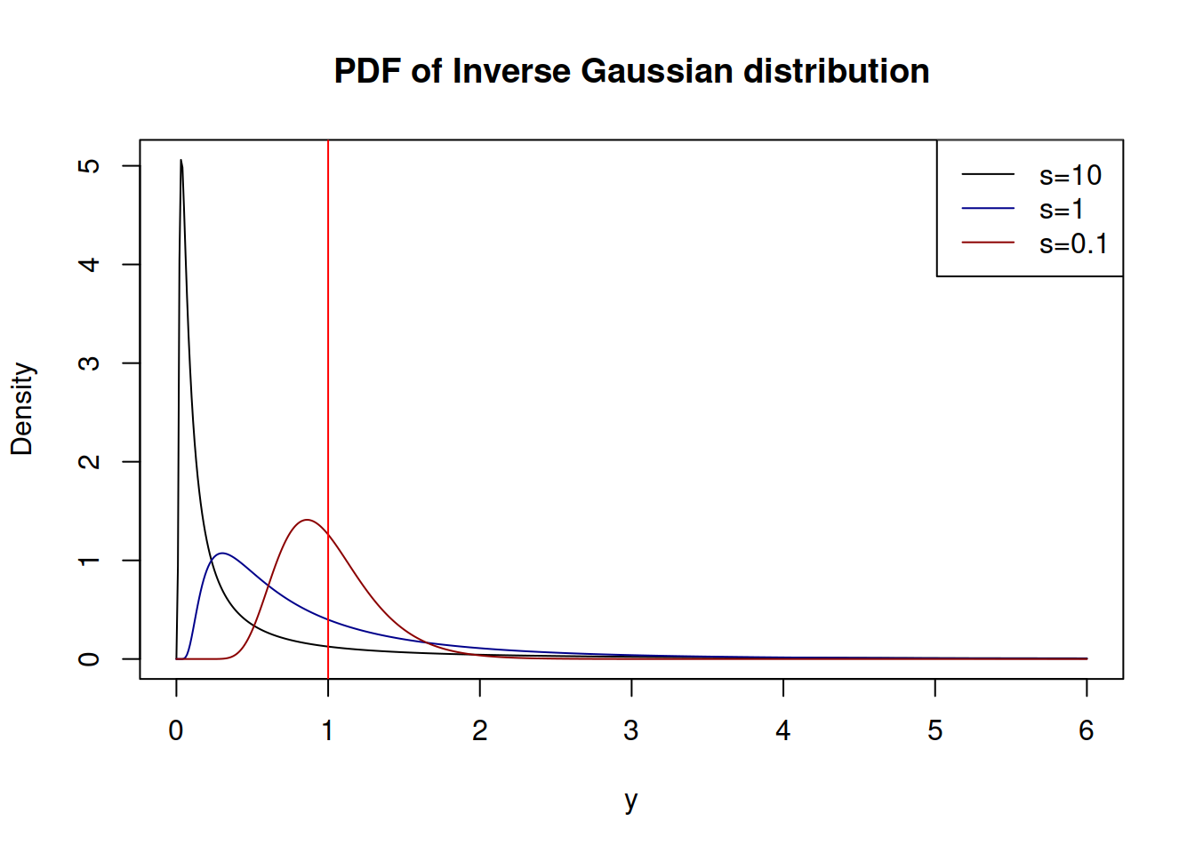
Figure 2.37: Probability Density Functions of Inverse Gaussian distribution
statmod package implements density, quantile, cumulative and random number generator functions for the \(\mathcal{IG}\).
2.7.8 Gamma distribution
Finally, another distribution that will be useful for ETS and ARIMA is Gamma (\(\mathcal{\Gamma}\)), which is parameterised using shape \(\xi\) and scale \(s\), and is defined for positive values only. This distribution is useful because it is scalable and is as flexible as (\(\mathcal{IG}\)) in terms of possible shapes. It also has an important scalability property (simila to \(\mathcal{IG}\)), but the shape needs to be restricted in order to make sense in ETS model: \[\begin{equation} \text{if } (1+\epsilon_t) \sim \mathcal{\Gamma}(s^{-1}, s) \text{, then } y_t = \mu_{y,t} \times (1+\epsilon_t) \sim \mathcal{\Gamma}\left(s^{-1}, s \mu_{y,t} \right), \tag{2.37} \end{equation}\] implying that the scale of the model changes together with the expectation. The restriction on the shape parameters is needed in order to make the expectation of \((1+\epsilon_t)\) equal to one. The PDF of the distribution of \(1+\epsilon_t\) is:
\[\begin{equation} f(1+\epsilon_t) = \frac{1}{\Gamma(s^{-1}) (s)^{s^{-1}}} (1+\epsilon_t)^{s^{-1}-1}\exp \left(-\frac{1+\epsilon_t}{s}\right) . \tag{2.38} \end{equation}\] However, the scale \(s\) cannot be estimated via the maximisation of likelihood analytically due to the restriction (2.37). Luckliy, the method of moments can be used instead, where based on the expectation and variance we get: \[\begin{equation} \hat{s} = \frac{1}{T} \sum_{t=1}^T e_t^2 , \tag{2.39} \end{equation}\] where \(e_t\) is the estimate of \(\epsilon_t\). So, imposing the restrictions (2.37) implies that the scale of \(\mathcal{\Gamma}\) is equal to the variance of the error term.
Figure 2.38 demonstrates how the PDF of \(\mathcal{\Gamma}(s^{-1},s)\) looks for different values of \(s\):
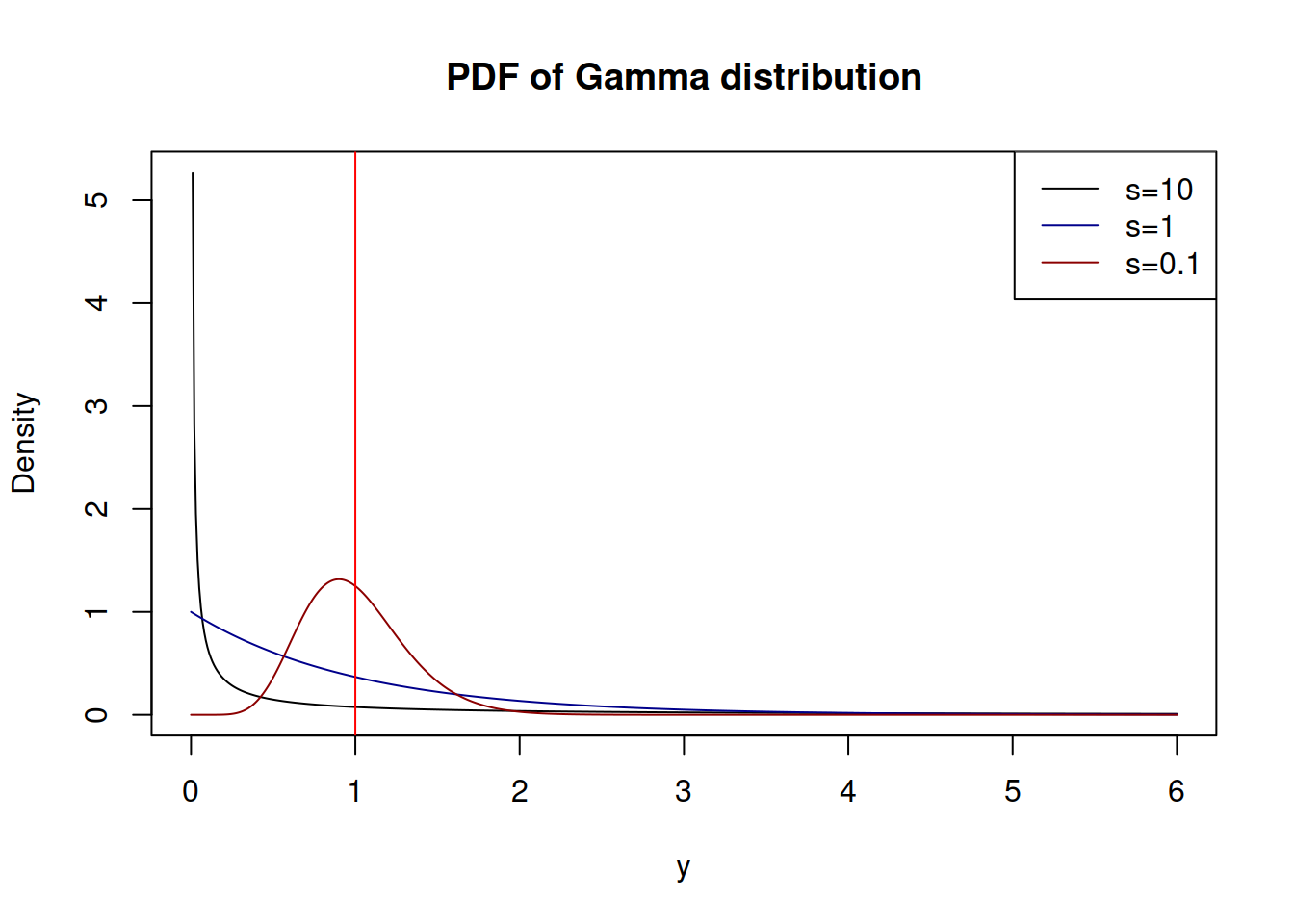
Figure 2.38: Probability Density Functions of Gamma distribution
With the increase of the shape \(\xi=s^{-1}\) (in our case this implies the decrease of variance \(s\)), \(\mathcal{\Gamma}\) distribution converges to the normal one with \(\mu=\xi s=1\) and variance \(\sigma^2=s\). This demonstrates indirectly that the estimate of the scale (2.39) maximises the likelihood of the function (2.38), although I do not have any proper proof of this.