2.4 Rolling origin
Remark. The text in this section is based on the vignette for the greybox package, written by the author of this monograph.
When there is a need to select the most appropriate forecasting model or method for the data, the forecaster usually splits the sample into two parts: in-sample (aka “training set”) and holdout sample (aka out-sample or “test set”). The model is estimated on the in-sample, and its forecasting performance is evaluated using some error measure on the holdout sample.
Using this procedure only once is known as “fixed origin” evaluation. However, this might give a misleading impression of the accuracy of forecasting methods. If, for example, the time series contains outliers or level shifts, a poor model might perform better in fixed origin evaluation than a more appropriate one just by chance. So it makes sense to have a more robust evaluation technique, where the model’s performance is evaluated several times, not just once. An alternative procedure known as “rolling origin” evaluation is one such technique.
In rolling origin evaluation, the forecasting origin is repeatedly moved forward by a fixed number of observations, and forecasts are produced from each origin (Tashman, 2000). This technique allows obtaining several forecast errors for time series, which gives a better understanding of how the models perform. This can be considered a time series analogue to cross-validation techniques (see Chapter 5 of James et al., 2017). Here is a simple graphical representation, courtesy of Nikos Kourentzes.
Figure 2.4: Visualisation of rolling origin by Nikos Kourentzes
The plot in Figure 2.4 shows how the origin moves forward and the point and interval forecasts of the model change. As a result, this procedure gives information about the performance of the model over a set of observations, not on a random one. There are different options of how this can be done, and here we discuss the main principles behind it.
2.4.1 Principles of rolling origin
Figure 2.5 (Svetunkov and Petropoulos, 2018) illustrates the basic idea behind rolling origin. White cells correspond to the in-sample data, while the light grey cells correspond to the three steps ahead forecasts. The time series in the figure has 25 observations, and forecasts are produced for eight origins starting from observation 15. In the first step, the model is estimated on the first in-sample set, and forecasts are created for the holdout. Next, another observation is added to the end of the in-sample set, the test set is advanced, and the procedure is repeated. The process stops when there is no more data left. This is a rolling origin with a constant holdout sample size. As a result of this procedure, eight one to three steps ahead forecasts are produced. Based on them, we can calculate the preferred error measures and choose the best performing model (see Section 2.1.2).
Figure 2.5: Rolling origin with constant holdout size from Svetunkov and Petropoulos, (2018).
Another option for producing forecasts via rolling origin would be to continue with rolling origin even when the test sample is smaller than the forecast horizon, as shown in Figure 2.6. In this case, the procedure continues until origin 22, when the last complete set of three steps ahead forecasts can be produced, and then continues with a decreasing forecasting horizon. So the two steps ahead forecast is produced from origin 23, and only a one-step-ahead forecast is produced from origin 24. As a result, we obtain ten one-step-ahead forecasts, nine two steps ahead forecasts and eight three steps ahead forecasts. This is a rolling origin with a non-constant holdout sample size, which can be helpful with small samples when not enough observations are available.
Figure 2.6: Rolling origin with non-constant holdout size.
Finally, in both cases above, we had the increasing in-sample size. However, we might need a constant in-sample for some research purposes. Figure 2.7 demonstrates such a setup. In this case, in each iteration, we add an observation to the end of the in-sample series and remove one from the beginning (dark grey cells).
Figure 2.7: Rolling origin with constant in-sample size.
2.4.2 Implementing rolling origin in R
Now that we discussed the main idea of rolling origin, we can see how it can be implemented in R. In this section, we will implement rolling origin with a fixed holdout sample size and a changing in-sample. This aligns with what is typically done in practice when new data arrives: the model is re-estimated, and forecasts are produced for the next \(h\) steps ahead. For this example, we will use artificially created data and apply a Simple Moving Average (discussed in Subsection 3.3.3) implemented in the smooth package.
We will produce forecasts for the horizon of 10 steps ahead, \(h=10\) from 5 origins.
We will create a list containing several objects of interest:
actualswill contain all the actual values;holdoutwill be a matrix containing the actual values for the holdout. It will havehrows andoriginscolumns;meanwill contain point forecasts from our model. This will also be a matrix with the same dimensions as theholdoutone.
returnedValues1 <- setNames(vector("list",3),
                            c("actuals","holdout","mean"))
returnedValues1$actuals <- y
returnedValues1$holdout <-
  returnedValues1$mean <-
  matrix(NA,h,origins,
         dimnames=list(paste0("h",1:h),
                       paste0("origin",1:origins)))
Finally, we write a simple loop that repeats the model fit and forecasting for the horizon h several times. The trickiest part is understanding how to define the train and test samples. In our example, the former should have obs+1-origins-h observations in the first step and obs-h in the last one so that we can have h observations in the test set throughout all origins, and we can repeat this origins times. One way of doing this is via the following loop:
for(i in 1:origins){
    # Fit the model
    testModel <- sma(y[1:(obs+i-origins-h)])
    # Drop the in-sample observations
    # and extract the first h observations from the rest
    returnedValues1$holdout[,i] <- head(y[-c(1:(obs-origins+i-h))], h)
    # Produce forecasts and write down the mean values
    returnedValues1$mean[,i] <- forecast(testModel, h=h)$mean
}
This basic loop can be amended to include anything else we want from the function or by changing the parameters of the rolling origin. After filling in the object returnedValues1, we can analyse the residuals of the model over the horizon and several origins in various ways. For example, Figure 2.8 shows boxplots across the horizon of 10 for different origins.
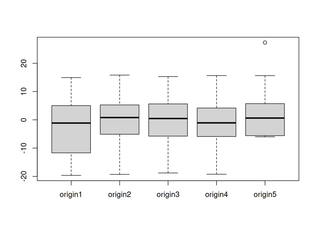
Figure 2.8: Boxplots of forecast errors over several origins.
In the ideal situation, the boxplots in Figure 2.8 should be similar, meaning that the model performs consistently over different origins. We do not see this in our case, observing that the distribution of errors changes from one origin to another.
While the example above already gives some information about the performance of a model, more useful information could be obtained if the performance of one model is compared to the others in the rolling origin experiment. This can be done manually for several models using the code above or it can be done using the function ro() from the greybox package.
2.4.3 Rolling origin function in R
In R, there are several packages and functions that implement rolling origin. One of those is the function ro() from the greybox package (written by Yves Sagaert and Ivan Svetunkov in 2016 on their way to the International Symposium on Forecasting in Riverside, US). It implements the rolling origin evaluation for any function you like with a predefined call and returns the desired value. It heavily relies on the two variables: call and value – so it is pretty important to understand how to formulate them to get the desired results. ro() is a very flexible function, but as a result, it is not very simple. In this subsection, we will see how it works in a couple of examples.
We start with a simple example, generating a series from Normal distribution:
We use an ARIMA(0,1,1) model implemented in the stats package (this model is discussed in Section 8). Given that we are interested in forecasts from the model, we need to use the predict() function to get the desired values:
The call that we specify includes two important elements: data and h. data specifies where the in-sample values are located in the function that we want to use, and it needs to be called “data” in the call; h will tell our function, where the forecasting horizon is specified in the provided line of code. Note that in this example we use arima(x=data,order=c(0,1,1)), which produces a desired ARIMA(0,1,1) model and then we use predict(..., n.ahead=h), which produces an \(h\) steps ahead forecast from that model.
Having the call, we also need to specify what the function should return. This can be the conditional mean (point forecasts), prediction intervals, the parameters of a model, or, in fact, anything that the model returns (e.g. name of the fitted model and its likelihood). However, there are some differences in what ro() returns depending on what the function returns. If it is a vector, then ro() will produce a matrix (with values for each origin in columns). If it is a matrix, then an array is returned. Finally, if it is a list, then a list of lists is returned.
In order not to overcomplicate things, we start with collecting the conditional mean from the predict() function:
Remark. If you do not specify the value to return, the function will try to return everything, but it might fail, especially if many values are returned. So, to be on the safe side, always provide the value when possible.
Now that we have specified ourCall and ourValue, we can produce forecasts from the model using rolling origin. Let’s say that we want three steps ahead forecasts and eight origins with the default values of all the other parameters:
The function returns a list with all the values that we asked for plus the actual values and the holdout sample. We can calculate some basic error measure based on those values, for example, scaled Absolute Error (Petropoulos and Kourentzes, 2015):
apply(abs(returnedValues1$holdout - returnedValues1$pred),
      1, mean, na.rm=TRUE) /
  mean(returnedValues1$actuals)
## h1 h2 h3
## 0.1067009 0.1005935 0.1079764In this example, we use the apply() function to distinguish between the different forecasting horizons and have an idea of how the model performs for each of them. These numbers do not tell us much on their own, but if we compare the performance of this model with an alternative one, we could infer if one model is more appropriate for the data than the other one. For example, applying ARIMA(0,2,2) to the same data, we will get:
ourCall <- "predict(arima(x=data,order=c(0,2,2)),n.ahead=h)"
returnedValues2 <- ro(y, h=3, origins=8,
                      call=ourCall, value=ourValue)
apply(abs(returnedValues2$holdout - returnedValues2$pred),
      1, mean, na.rm=TRUE) /
  mean(returnedValues2$actuals)
## h1 h2 h3
## 0.10691559 0.09491994 0.10595135Comparing these errors with the ones from the previous model, we can conclude which of the approaches is more suitable for the data.
We can also plot the forecasts from the rolling origin, which shows how the models behave:
par(mfcol=c(2,1), mar=c(4,4,3,1))
plot(returnedValues1, main="ARIMA(0,1,1)")
plot(returnedValues2, main="ARIMA(0,2,2)")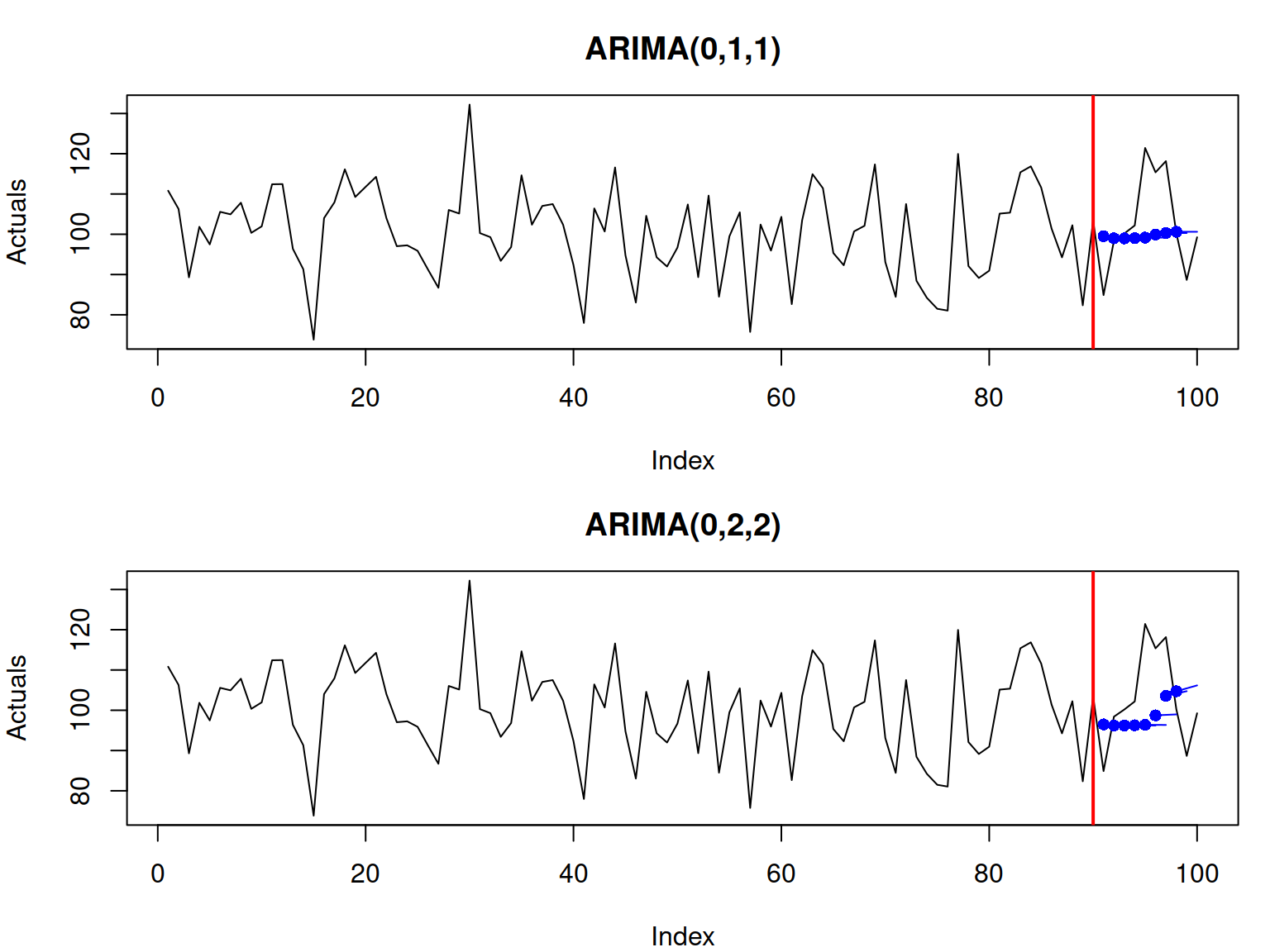
Figure 2.9: Rolling origin performance of two forecasting methods.
In Figure 2.9, the forecasts from different origins are close to each other. This is because the data is stationary, and both models produce flat lines as forecasts. The second model, however, has a slightly higher variability because it has more parameters than the first one (bias-variance trade-off in action).
The rolling origin function from the greybox package also allows working with explanatory variables and returning prediction intervals if needed. Some further examples are discussed in the vignette of the package. Just run the command vignette("ro","greybox") in R to see it.
Practically speaking, if we have a set of forecasts from different models we can analyse the distribution of error measures and come to conclusions about the performance of models. Here is an example with an analysis of performance for \(h=1\) based on absolute errors:
aeValuesh1 <- cbind(abs(returnedValues1$holdout -
                          returnedValues1$pred)[1,],
                    abs(returnedValues1$holdout -
                          returnedValues2$pred)[1,])
colnames(aeValuesh1) <- c("ARIMA(0,1,1)","ARIMA(0,2,2)")
boxplot(aeValuesh1)
points(apply(aeValuesh1,2,mean),pch=16,col="red")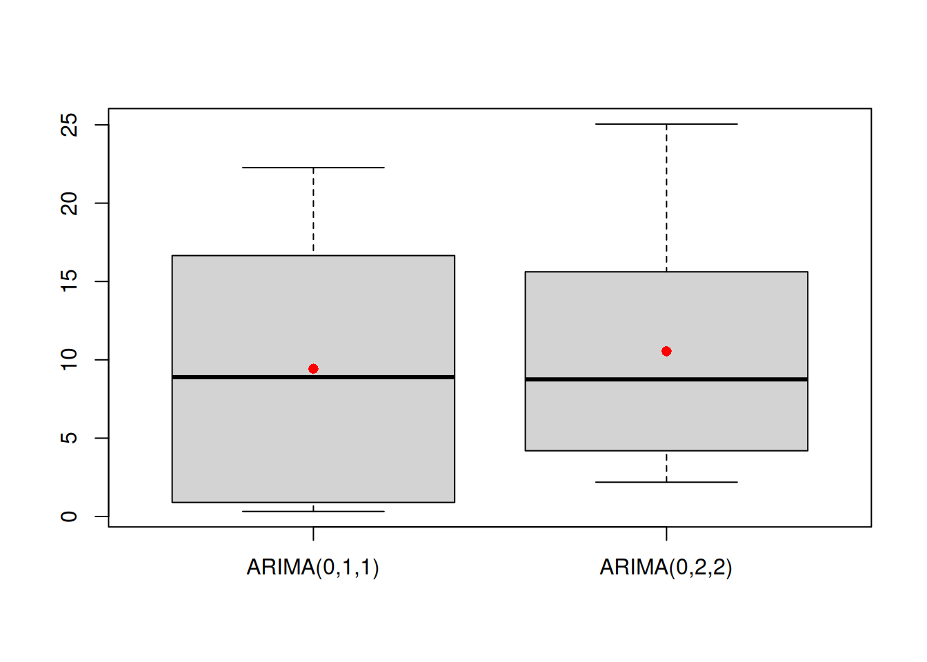
Figure 2.10: Boxplots of error measures of two methods.
The boxplots in Figure 2.10 can be interpreted as any other boxplot applied to random variables (see, for example, discussion in Section 5.2 of Svetunkov and Yusupova, 2025).
Remark. When it comes to applying ro() to models with explanatory variables, one can use the internal parameters counti, counto, and countf, which define the size of the in-sample, the holdout and the full sample, respectively. An example of the code in this situation is shown below with a function alm() from the greybox package being used for fitting a simple linear regression model.
# Generate the data
x <- rnorm(100, 100, 10)
xreg <- cbind(y=100+1.5*x+rnorm(100, 0, 10), x=x)
# Predict values from the model.
# counti and counto determine sizes for the in-sample and the holdout
ourCall <- "predict(alm(y~x, data=xreg[counti,,drop=FALSE]),
                        newdata=xreg[counto,,drop=FALSE])"
# Extract the mean only
ourValue <- "mean"
# Run rolling origin
testRO <- ro(xreg[,"y"],h=5,origins=5,ourCall,ourValue)
# plot the result
plot(testRO)