3.6 Statistical models assumptions
In order for a statistical model to work adequately and not to fail, when applied to a data, several assumptions about it should hold. If they do not, then the model might lead to biased or inefficient estimates of parameters and inaccurate forecasts. In this section we discuss the main assumptions, united in three big groups:
- Model is correctly specified;
- Residuals are independent and identically distributed (i.i.d.);
- The explanatory variables are not correlated with anything but the response variable.
We do not aim to explain why the violation of assumptions would lead to the discussed problem, and refer a curious reader to econometrics textbooks (for example Hanck et al., 2020). In many cases, in our discussions in this textbook, we assume that all of these assumptions hold. In some of the cases, we will say explicitly, which are violated and what needs to be done in those situations. In Section 17 we will discuss how these assumptions can be checked for dynamic models, and how the issues caused by their violation can be fixed.
3.6.1 Model is correctly specified
This is one of the fundamental group of assumptions, which can be summarised as “we have included everything necessary in the model in the correct form.” It implies that:
- We have not omitted important variables in the model (underfitting the data);
- We do not have redundant variables in the model (overfitting the data);
- The necessary transformations of the variables are applied;
- We do not have outliers in the model.
3.6.1.1 Omitted variables
If there are some important variables that we did not include in the model, then the estimates of the parameters might be biased and in some cases quite seriously (e.g. positive sign instead of the negative one). A classical example of model with omitted important variables is simple linear regression, which by definition includes only one explanatory variable. Making decisions based on such model might not be wise, as it might mislead about the significance and sign of effects. Yes, we use simple linear regression for educational purposes, to understand how the model works and what it implies, but it is not sufficient on its own. Finally, when it comes to forecasting, omitting important variables is equivalent to underfitting the data, ignoring significant aspects of the model. This means that the point forecasts from the model might be biased (systematic under or over forecasting), the variance of the error term will be higher than needed, which will result in wider than necessary prediction interval.
In some cases, it is possible to diagnose the violation of this assumption. In order to do that an analyst needs to analyse a variety of plots of residuals vs fitted, vs time (if we deal with time series), and vs omitted variables. Consider an example with mtcars data and a simple linear regression:
mtcarsSLR <- alm(mpg~wt, mtcars, loss="MSE")Based on the preliminary analysis that we have conducted in Sections 2.1 and 2.6, this model omits important variables. And there are several basic plots that might allow us diagnosing the violation of this assumption.
par(mfcol=c(1,2))
plot(mtcarsSLR,c(1,2))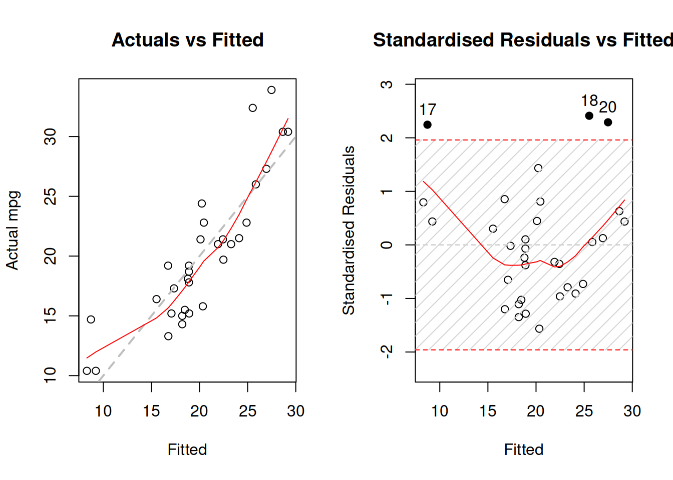
Figure 3.29: Diagnostics of omitted variables.
Figure 3.29 demonstrates actuals vs fitted and fitted vs standardised residuals. The standardised residuals are the residuals from the model that are divided by their standard deviation, thus removing the scale. What we want to see on the first plot in Figure 3.29, is for all the point lie around the grey line and for the LOWESS line to coincide with the grey line. That would mean that the relations are captured correctly and all the observations are explained by the model. As for the second plot, we want to see the same, but it just presents that information in a different format, which is sometimes easier to analyse. In both plot of Figure 3.29, we can see that there are still some patterns left: the LOWESS line has a u-shaped form, which in general means that something is wrong with model specification. In order to investigate if there are any omitted variables, we construct a spread plot of residuals vs all the variables not included in the model (Figure 3.30).
spread(data.frame(residuals=resid(mtcarsSLR), mtcars[,-c(1,6)]))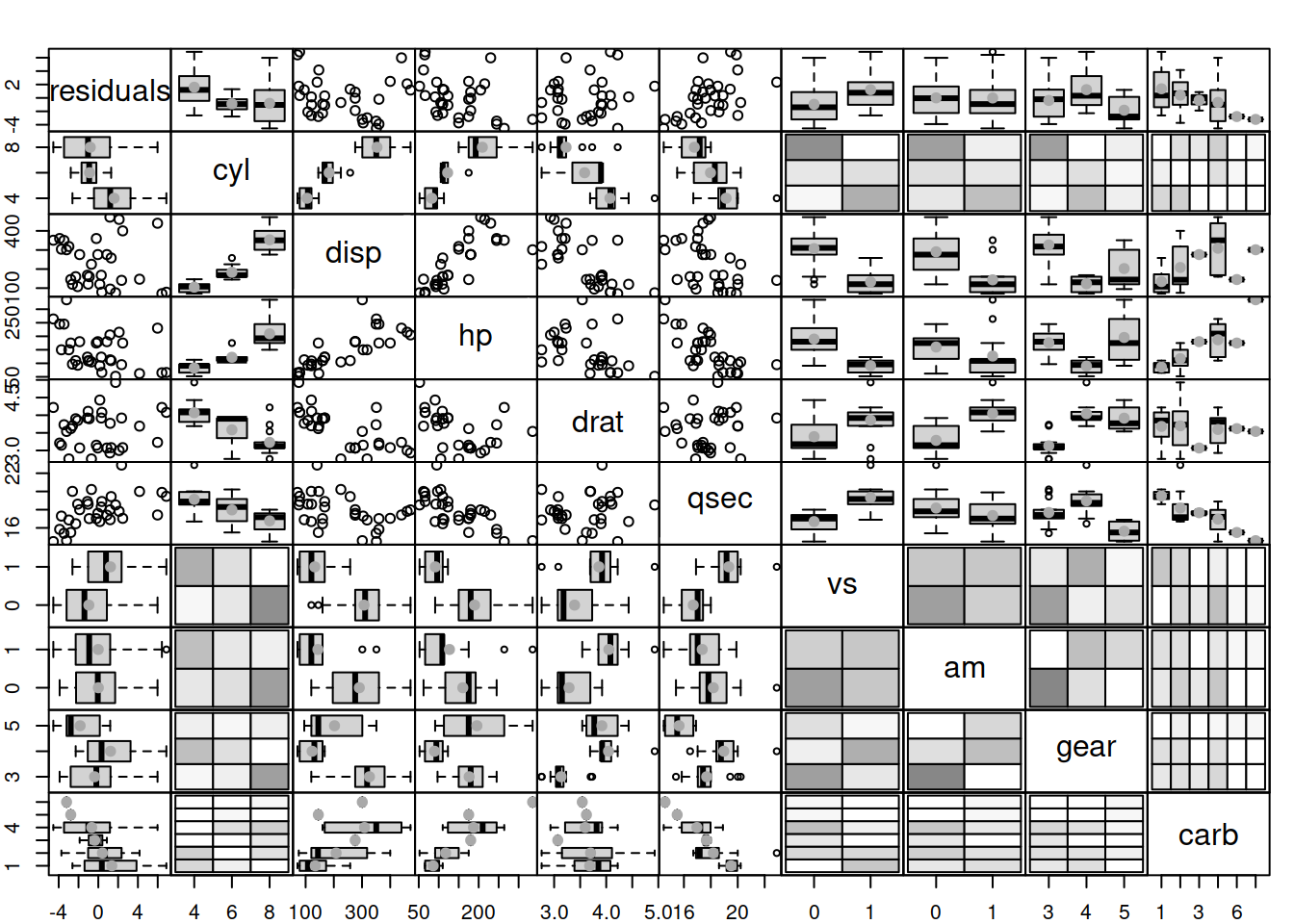
Figure 3.30: Diagnostics of omitted variables.
What we want to see in Figure 3.30 is the absence of any patterns in plots of residuals vs variables. However, we can see that there are still many relations. For example, with the increase of the number of cylinders, the mean of residuals decreases. This might indicate that the variable is needed in the model. And indeed, we can imagine a situation, where mileage of a car (the response variable in our model) would depend on the number of cylinders because the bigger engines will have more cylinders and consume more fuel, so it makes sense to include this variable in the model as well.
Note that we do not suggest to start modelling from simple linear relation! You should construct a model that you think is suitable for the problem, and the example above is provided only for illustrative purposes.
3.6.1.2 Redundant variables
If there are redundant variables that are not needed in the model, then the estimates of parameters and point forecasts might be unbiased, but inefficient. This implies that the variance of parameters can be lower than needed and thus the prediction intervals will be narrower than needed. There are no good instruments for diagnosing this issue, so judgment is needed, when deciding what to include in the model.
3.6.1.3 Transformations
This assumption implies that we have taken all possible non-linearities into account. If, for example, instead of using a multiplicative model, we apply an additive one, the estimates of parameters and the point forecasts might be biased. This is because the model will produce linear trajectory of the forecast, when a non-linear one is needed. This was discussed in detail in Section 3.5. The diagnostics of this assumption is similar to the diagnostics shown above for the omitted variables: construct actuals vs fitted and residuals vs fitted in order to see if there are any patterns in the plots. Take the multiple regression model for mtcars, which includes several variables, but is additive in its form:
mtcarsALM01 <- alm(mpg~wt+qsec+am, mtcars, loss="MSE")Arguably, the model includes important variables (although there might be some others that could improve it), but the residuals will show some patterns, because the model should be multiplicative (see Figure 3.31), because mileage should not reduce linearly with increase of those variables. In order to understand that, ask yourself, whether the mileage can be negative and whether weight and other variables can be non-positive (a car with \(wt=0\) just does not exist).
par(mfcol=c(1,2))
plot(mtcarsALM01,c(1,2))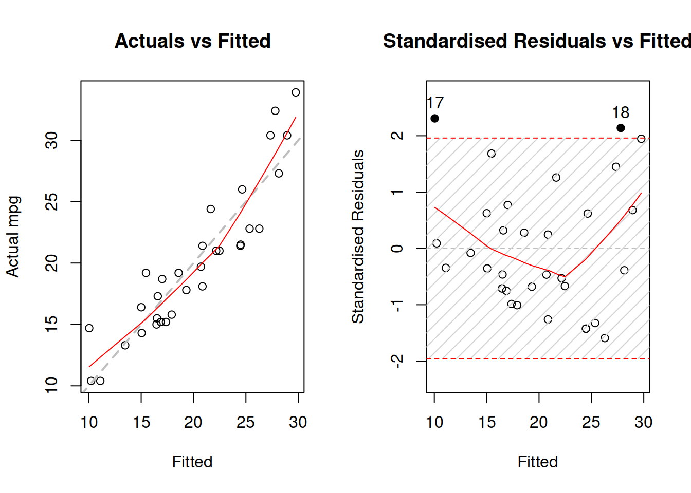
Figure 3.31: Diagnostics of necessary transformations in linear model.
Figure 3.31 demonstrates the u-shaped pattern in the residuals, which is one of the indicators of a wrong model specification, calling for a non-linear transformation. We can try a model in logarithms:
mtcarsALM02 <- alm(log(mpg)~log(wt)+log(qsec)+am, mtcars, loss="MSE")And see what would happen with the diagnostics of the model in logarithms:
par(mfcol=c(1,2))
plot(mtcarsALM02,c(1,2))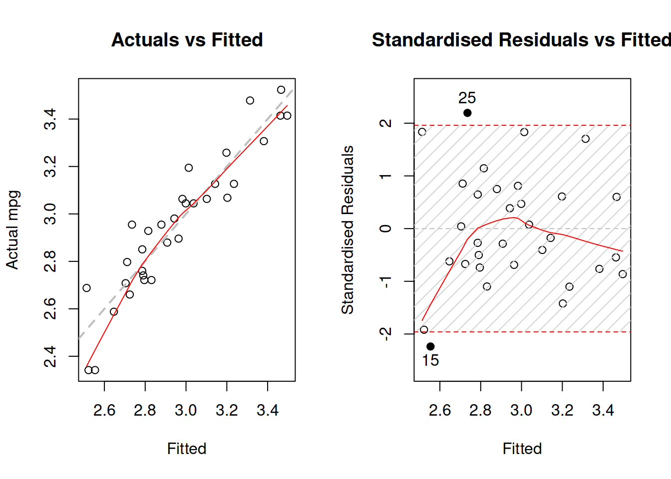
Figure 3.32: Diagnostics of necessary transformations in log-log model.
Figure 3.32 demonstrates that while the LOWESS lines do not coincide with the grey lines, the residuals do not have obvious patterns. The fact that the LOWESS line starts from below, when fitted values are low in our case only shows that we do not have enough observations with low actual values. As a result, LOWESS is impacted by 2 observations that lie below the grey line. This demonstrates that LOWESS lines should be taken with a pinch of salt and we should abstain from finding patterns in randomness, when possible. Overall, the log-log model is more appropriate to this data than the linear one.
3.6.1.4 Outliers
In a way, this assumption is similar to the first one with omitted variables. The presence of outliers might mean that we have missed some important information, implying that the estimates of parameters and forecasts would be biased. There can be other reasons for outliers as well. For example, we might be using a wrong distributional assumption. If so, this would imply that the prediction interval from the model is narrower than necessary. The diagnostics of outliers comes to producing standardised residuals vs fitted, to studentised vs fitted and to Cook’s distance plot. While we are already familiar with the first one, the other two need to be explained in more detail.
Studentised residuals are the residuals that are calculated in the same way as the standardised ones, but removing the value of each residual. For example, the studentised residual on observation 25 would be calculated as the raw residual divided by standard deviation of residuals, calculated without this 25th observation. This way we diminish the impact of potential serious outliers on the standard deviation, making it easier to spot the outliers.
As for the Cook’s distance, its idea is to calculate measures for each observation showing how influential they are in terms of impact on the estimates of parameters of the model. If there is an influential outlier, then it would distort the values of parameters, causing bias.
par(mfcol=c(1,2))
plot(mtcarsALM02,c(2,3))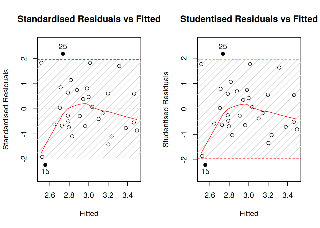
Figure 3.33: Diagnostics of outliers.
Figure 3.33 demonstrates standardised and studentised residuals vs fitted values for the log-log model on mtcars data. We can see that the plots are very similar, which already indicates that there are no strong outliers in the residuals. The bounds produced on the plots correspond to the 95% prediction interval, so by definition it should contain \(0.95\times 32 \approx 30\) observations. Indeed, there are only two observations: 15 and 25 - that lie outside the bounds. Technically, we would suspect that they are outliers, but they do not lie far away from the bounds and their number meets our expectations, so we can conclude that there are no outliers in the data.
plot(mtcarsALM02,12)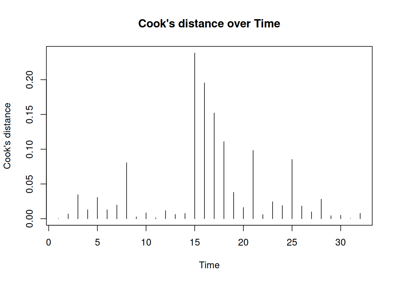
Figure 3.34: Cook’s distance plot.
Finally, we produce Cook’s distance over observations in Figure 3.34. The x-axis says “Time,” because alm() function is tailored for time series data, but this can be renamed into “observations.” The plot shows how influential the outliers are. If there were some significantly influential outliers in the data, then the plot would draw red lines, corresponding to 0.5, 0.75 and 0.95 quantiles of Fisher’s distribution, and the line of those outliers would be above the red lines. Consider the following example for demonstration purposes:
mtcarsData[28,6] <- 4
mtcarsALM03 <- alm(log(mpg)~log(wt)+log(qsec)+am, mtcarsData, loss="MSE")
This way, we intentionally create an influential outlier (the car should have the minimum weight in the dataset, and now it has a very high one).
plot(mtcarsALM03, 12, ylim=c(0,1.5), xlab="Observations", main="")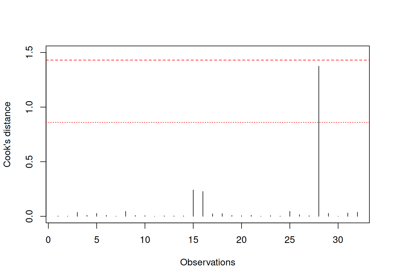
Figure 3.35: Cook’s distance plot for the data with influential outlier.
Figure 3.35 shows how Cook’s distance will look in this case - it detects that there is an influential outlier, which is above the norm. We can compare the parameters of the new and the old models to see how the introduction of one outlier leads to bias in the estimates of parameters:
rbind(coef(mtcarsALM02),
      coef(mtcarsALM03))
## (Intercept) log(wt) log(qsec) am
## [1,] 1.2095788 -0.7325269 0.8857779 0.05205307
## [2,] 0.1382442 -0.4852647 1.1439862 0.214063313.6.2 Residuals are i.i.d.
There are five assumptions in this group:
- There is no autocorrelation in the residuals;
- The residuals are homoscedastic;
- The expectation of residuals is zero, no matter what;
- The variable follows the assumed distribution;
- More generally speaking, distribution of residuals does not change over time.
3.6.2.1 No autocorrelations
This assumption only applied to time series data, and in a way comes to capturing correctly the dynamic relations between variables. The term “autocorrelation” refers to the situation, when variable is correlated with itself from the past. If the residuals are autocorrelated, then something is neglected by the applied model. Typically, this leads to inefficient estimates of parameters, which in some cases might also become biased. The model with autocorrelated residuals might produce inaccurate point forecasts and prediction intervals of a wrong width (wider or narrower than needed).
There are several ways of diagnosing the problem, including visual analysis and statistical tests. In order to show some of them, we consider the Seatbelts data from datasets package for R. We fit a basic model, predicting monthly totals of car drivers in the Great Britain killed or seriously injured in car accidents:
SeatbeltsALM01 <- alm(drivers~PetrolPrice+kms+front+rear+law, Seatbelts)In order to do graphical diagnose, we can produce plots of standardised / studentised residuals over time:
plot(SeatbeltsALM01,8,main="")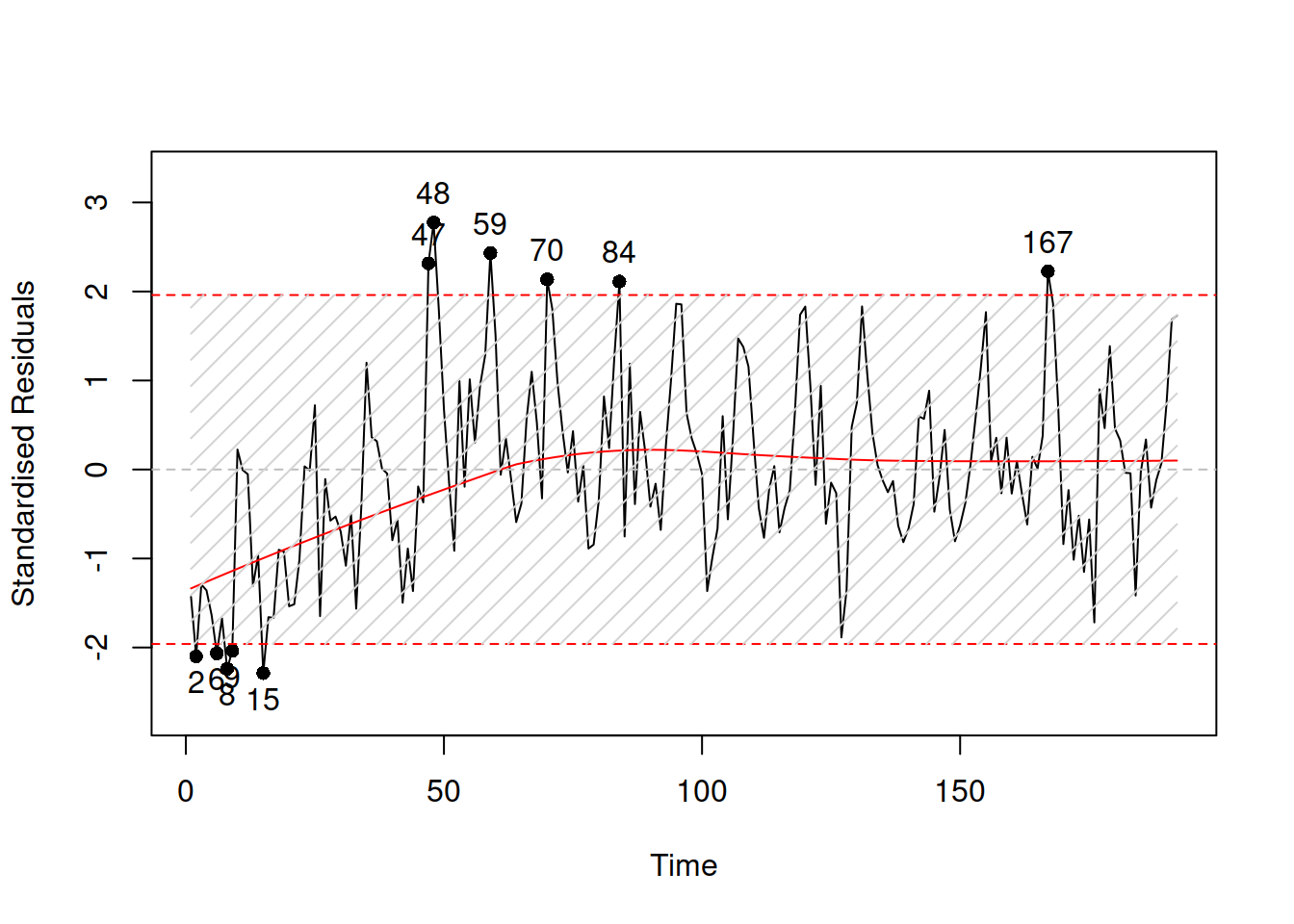
Figure 3.36: Standardised residuals over time.
If the assumption is not violated, then the plot in Figure 3.36 would not contain any patterns. However, we can see that, first, there is a seasonality in the residuals and second, the expectation (captured by the red LOWESS line) changes over time. This indicates that there might be some autocorrelation in residuals caused by omitted components. We do not aim to resolve the issue now, it is discussed in more detail in Section 17.5.
The other instrument for diagnostics is ACF / PACF plots, which are produced in alm() via the following command:
par(mfcol=c(1,2))
plot(SeatbeltsALM01,c(10,11),main="")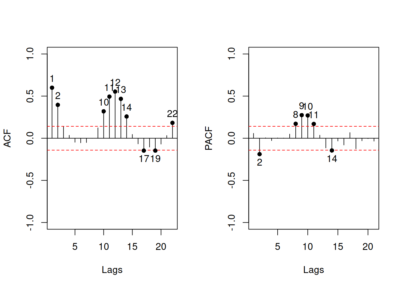
Figure 3.37: ACF and PACF of the residuals of a model.
These are discussed in more detail in Sections 11.3.2 and 11.3.3.
3.6.2.2 Homoscedastic residuals
In general, we assume that the variance of residuals is constant. If this is violated, then we say that there is a heteroscedasticity in the model. This means that with a change of a variable, the variance of the residuals will change as well. If the model neglects this, then typically the estimates of parameters become inefficient and prediction intervals are wrong: they are wider than needed in some cases (e.g.m when the volume of data is low) and narrower than needed in the other ones (e.g. on high volume data).
Typically, this assumption will be violated if the model is not specified correctly. The classical example is the income versus expenditure on meals for different families. If the income is low, then there is not many options what to buy and the variability of expenditures would be low. However, with the increase of the income, the mean expenditures and their variability would increase as well, because there are more options of what to buy, including both cheap and expensive products. If we constructed a basic linear model on such data, then it would violate the assumption of homoscedasticity and as a result will have the issues discussed above. But arguably this would typically appear because of the misspecification of the model. For example, taking logarithms might resolve the issue in many cases, implying that the effect of one variable on the other should be multiplicative rather than the additive. Alternatively, dividing variables by some other variable (e.g. working with expenses per family member, not per family) might resolve the problem as well. Unfortunately, the transformations are not the panacea, so in some cases analyst would need to construct a model, taking the changing variance into account (e.g. GARCH or GAMLSS models). This is discussed in Section ??.
While in forecasting we are more interested in the holdout performance of models, in econometrics, the parameters of models are typically of the main interest. And, as we discussed earlier, in case of correctly specified model with heteroscedastic residuals, the estimates of parameters will be unbiased, but inefficient. So, econometricians would use different approaches to diminish the heteroscedasticity effect on parameters: either a different estimator for a model (such as Weighted Least Squares), or a different method for calculation of standard errors of parameters (e.g. Heteroskedasticity-Consistent Standard Errors). This does not resolve the problem, but rather corrects the parameters of the model (i.e. does not heal the illness, but treats the symptoms). Although these approaches typically suffice for the analytical purposes, they do not fix the issues in forecasting.
The diagnostics of heteroscedasticity can be done via plotting absolute and / or squared residuals against the fitted values.
par(mfcol=c(1,2))
plot(mtcarsALM01,4:5)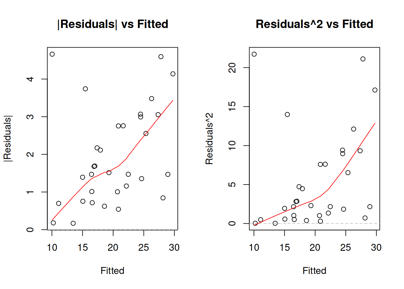
Figure 3.38: Detecting heteroscedasticity. Model 1.
If your model assumes that residuals follow a distribution related to the Normal one, then you should focus on the plot of squared residuals vs fitted, as this would be closer related to the variance of the distribution. In the example of mtcars model in Figure 3.38 we see that the variance of residuals increases with the increase of Fitted values (the LOWESS line increases and the overall variability around 1200 is lower than the one around 2000). This indicates that the residuals are heteroscedastic. One of the possible solutions of the problem is taking the logarithms, as we have done in the model mtcarsALM02:
par(mfcol=c(1,2))
plot(mtcarsALM02,4:5)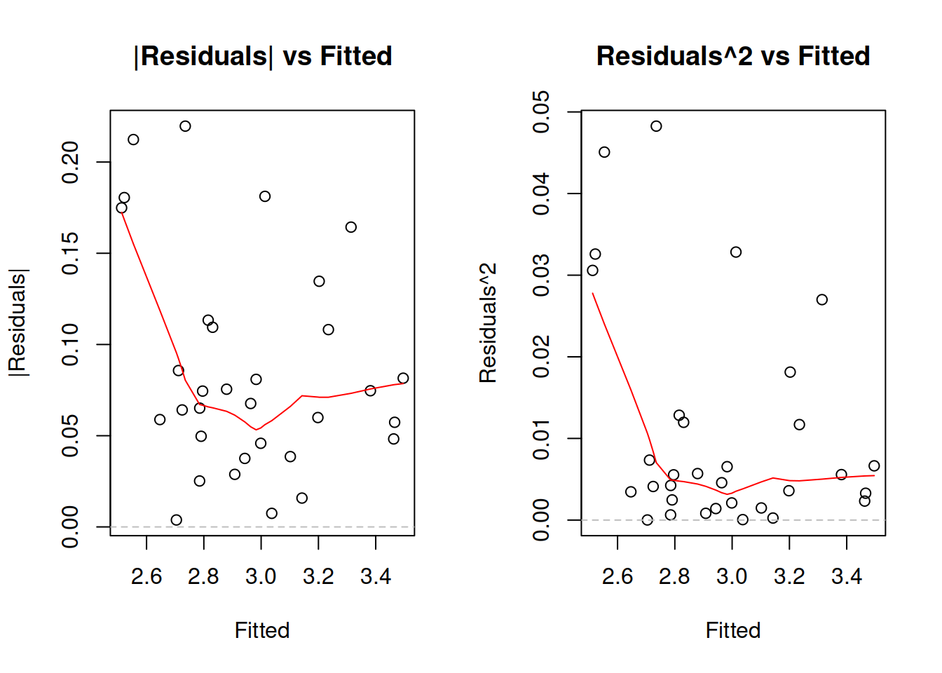
Figure 3.39: Detecting heteroscedasticity. Model 2.
While the LOWESS lines on plots in Figure 3.39 demonstrate some dynamics, the variability of residuals does not change significantly with the increase of fitted value, so non-linear transformation seems to fix the issue in our example. If it would not, then we would need to consider either some other transformations or finding out, which of the variables causes heteroscedasticity and then modelling it explicitly via the scale model (Section ??).
3.6.2.3 Mean of residuals
While in sample, this holds automatically in many cases (e.g. when using Least Squares method for regression model estimation), this assumption might be violated in the holdout sample. In this case the point forecasts would be biased, because they typically do not take the non-zero mean of forecast error into account, and the prediction interval might be off as well, because of the wrong estimation of the scale of distribution (e.g. variance is higher than needed). This assumption also implies that the expectation of residuals is zero even conditional on the explanatory variables in the model. If it is not, then this might mean that there is still some important information omitted in the applied model.
Note that some models assume that the expectation of residuals is equal to one instead of zero (e.g. multiplicative error models). The idea of the assumption stays the same, it is only the value that changes.
The diagnostics of the problem would be similar to the case of non-linear transformations or autocorrelations: plotting residuals vs fitted or residuals vs time and trying to find patterns. If the mean of residuals changes either with the change of fitted values of with time, then the conditional expectation of residuals is not zero, and something is missing in the model.
3.6.2.4 Distributional assumptions
In some cases we are interested in using methods that imply specific distributional assumptions about the model and its residuals. For example, it is assumed in the classical linear model that the error term follows Normal distribution. Estimating this model using MLE with the probability density function of Normal distribution or via minimisation of Mean Squared Error (MSE) would give efficient and consistent estimates of parameters. If the assumption of normality does not hold, then the estimates might be inefficient and in some cases inconsistent. When it comes to forecasting, the main issue in the wrong distributional assumption appears, when prediction intervals are needed: they might rely on a wrong distribution and be narrower or wider than needed. Finally, if we deal with the wrong distribution, then the model selection mechanism might be flawed and would lead to the selection of an inappropriate model.
The most efficient way of diagnosing this, is constructing QQ-plot of residuals (discussed in Section 2.1.2).
plot(mtcarsALM02,6)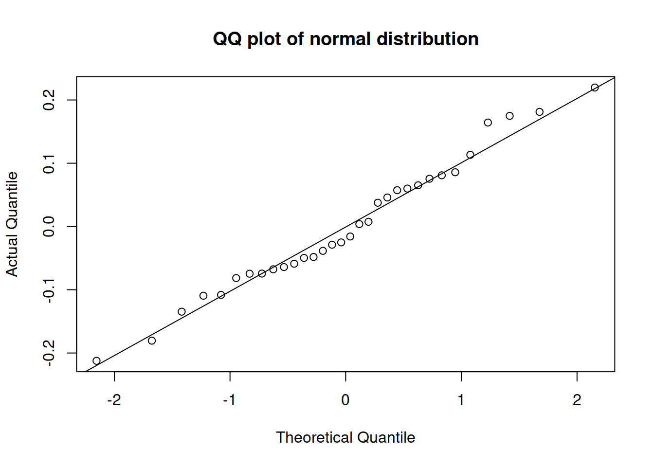
Figure 3.40: QQ-plot of residuals of model 2 for mtcars dataset.
Figure 3.40 shows that all the points lie close to the line (with minor fluctuations around it), so we can conclude that the residuals follow the normal distribution. In comparison, Figure 3.40 demonstrates how residuals would look in case of a wrong distribution. Although the values lie not too far from ths straight line, there are several observations in the tails that are further away than needed. Comparing the two plots, we would select the on in Figure 3.40, as the residuals are better behaved.
plot(mtcarsALM01,6)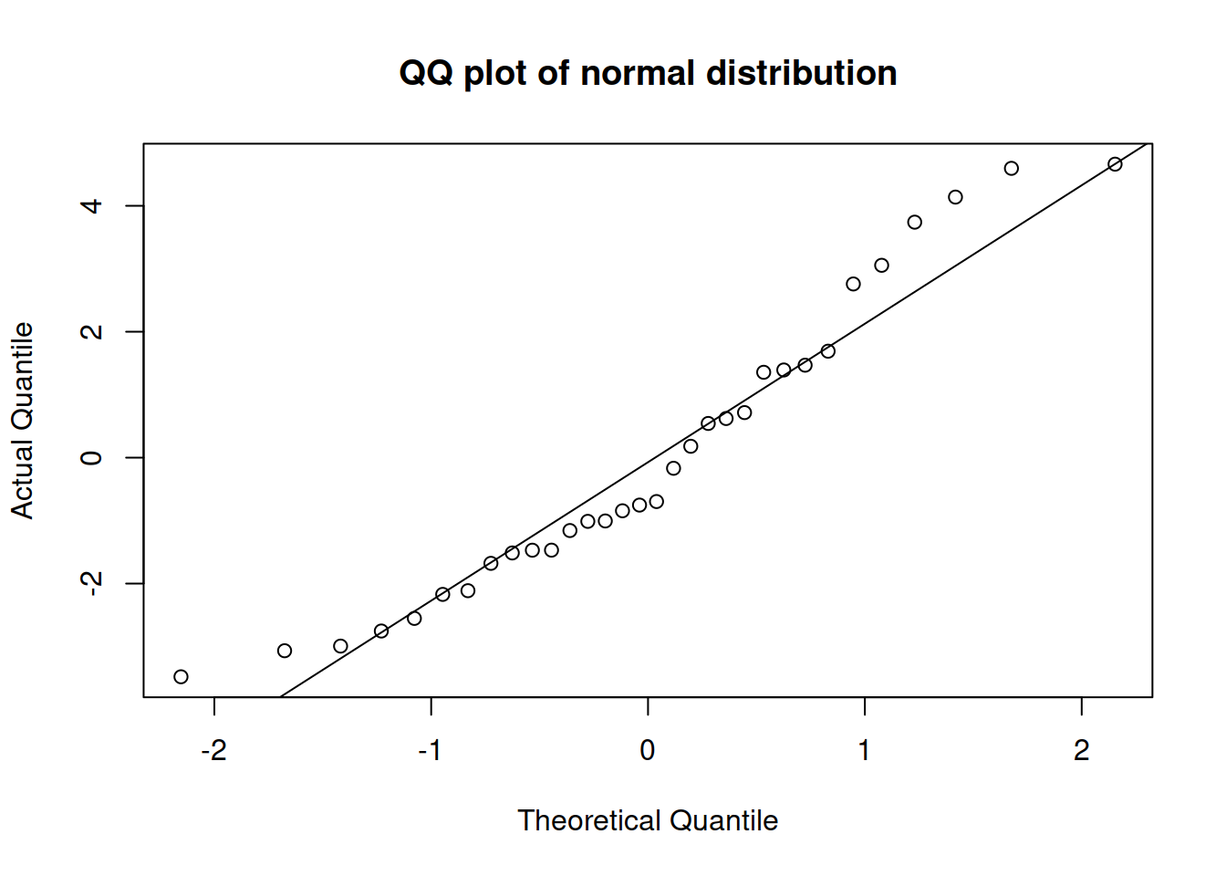
Figure 3.41: QQ-plot of residuals of model 1 for mtcars dataset.
3.6.2.5 Distribution does not change
This assumption aligns with the Subsection 3.6.2.4, but in this specific context implies that all the parameters of distribution stay the same and the shape of distribution does not change. If the former is violated then we might have one of the issues discussed above. If the latter is violated then we might produce biased forecasts and underestimate / overestimate the uncertainty about the future. The diagnosis of this comes to analysing QQ-plots, similar to Subsection 3.6.2.4.
3.6.3 The explanatory variables are not correlated with anything but the response variable
There are two assumptions in this group:
- No multicollinearity;
- No endogeneity;
3.6.3.1 Multicollinearity
One of the classical issues in econometrics and in statistics in regression context is the issue of multicollinearity, the effect when several explanatory variables are correlated. In a way, this has nothing to do with classical assumptions of linear regression, because it is unreasonable to assume that the explanatory variables have some specific relation between them - they are what they are, and multicollinearity mainly causes issues with estimation of the parameters of model, not with its structure. But it is an issue nonetheless, so it is worth exploring.
Multicollinearity appears, when either some of explanatory variables are correlated with each other (see Section 2.6.3), or their linear combination explains another explanatory variable included in the model. Depending on the strength of this relation and the estimation method used for model construction, the multicollinearity might cause issues of varying severity. For example, in the case, when two variables are perfectly correlated (correlation coefficient is equal to 1 or -1), the model will have perfect multicollinearity and it would not be possible to estimate its parameters. Another example is a case, when an explanatory variable can be perfectly explained by a set of other explanatory variables (resulting in \(R^2\) being close to one), which will cause exactly the same issue. The classical example of this situation is the dummy variables trap (see Section 3.4), when all values of categorical variable are included in regression together with the constant resulting in the linear relation \(\sum_{j=1}^k d_j = 1\). Given that the square root of \(R^2\) of linear regression is equal to multiple correlation coefficient, these two situations are equivalent and just come to “absolute value of correlation coefficient is equal to 1.” Finally, if correlation coefficient is high, but not equal to one, the effect of multicollinearity will lead to less efficient estimates of parameters. The loss of efficiency is in this case proportional to the absolute value of correlation coefficient. In case of forecasting, the effect is not as straight forward, and in some cases might not damage the point forecasts, but can lead to prediction intervals of an incorrect width. The main issue of multicollinearity comes to the difficulties in the model estimation in a sample. If we had all the data in the world, then the issue would not exist. All of this tells us how this problem can be diagnosed and that this diagnosis should be carried out before constructing regression model.
First, we can calculate correlation matrix for the available variables. If they are all numeric, then cor() function from stats should do the trick (we remove the response variable from consideration):
cor(mtcars[,-1])## cyl disp hp drat wt qsec
## cyl 1.0000000 0.9020329 0.8324475 -0.69993811 0.7824958 -0.59124207
## disp 0.9020329 1.0000000 0.7909486 -0.71021393 0.8879799 -0.43369788
## hp 0.8324475 0.7909486 1.0000000 -0.44875912 0.6587479 -0.70822339
## drat -0.6999381 -0.7102139 -0.4487591 1.00000000 -0.7124406 0.09120476
## wt 0.7824958 0.8879799 0.6587479 -0.71244065 1.0000000 -0.17471588
## qsec -0.5912421 -0.4336979 -0.7082234 0.09120476 -0.1747159 1.00000000
## vs -0.8108118 -0.7104159 -0.7230967 0.44027846 -0.5549157 0.74453544
## am -0.5226070 -0.5912270 -0.2432043 0.71271113 -0.6924953 -0.22986086
## gear -0.4926866 -0.5555692 -0.1257043 0.69961013 -0.5832870 -0.21268223
## carb 0.5269883 0.3949769 0.7498125 -0.09078980 0.4276059 -0.65624923
## vs am gear carb
## cyl -0.8108118 -0.52260705 -0.4926866 0.52698829
## disp -0.7104159 -0.59122704 -0.5555692 0.39497686
## hp -0.7230967 -0.24320426 -0.1257043 0.74981247
## drat 0.4402785 0.71271113 0.6996101 -0.09078980
## wt -0.5549157 -0.69249526 -0.5832870 0.42760594
## qsec 0.7445354 -0.22986086 -0.2126822 -0.65624923
## vs 1.0000000 0.16834512 0.2060233 -0.56960714
## am 0.1683451 1.00000000 0.7940588 0.05753435
## gear 0.2060233 0.79405876 1.0000000 0.27407284
## carb -0.5696071 0.05753435 0.2740728 1.00000000This matrix tells us that there are some variables that are highly correlated and might reduce efficiency of estimates of parameters of regression model if included in the model together. This mainly applies to cyl and disp, which both characterise the size of engine. If we have a mix of numerical and categorical variables, then assoc() (aka association()) function from greybox will be more appropriate (see Section 2.6).
assoc(mtcars)In order to cover the second situation with linear combination of variables, we can use the determ() (aka determination()) function from greybox:
determ(mtcars[,-1])## cyl disp hp drat wt qsec vs am
## 0.9349544 0.9537470 0.8982917 0.7036703 0.9340582 0.8671619 0.7986256 0.7848763
## gear carb
## 0.8133441 0.8735577This function will construct linear regression models for each variable from all the other variables and report the \(R^2\) from these models. If there are coefficients of determination close to one, then this might indicate that the variables would cause multicollinearity in the model. In our case, we see that disp is linearly related to other variables, and we can expect it to cause the reduction of efficiency of estimate of parameters. If we remove it from the consideration (we do not want to include it in our model anyway), then the picture will change:
determ(mtcars[,-c(1,3)])## cyl hp drat wt qsec vs am gear
## 0.9299952 0.8596168 0.6996363 0.8384243 0.8553748 0.7965848 0.7847198 0.8121855
## carb
## 0.7680136Now cyl has linear relation with some other variables, so it would not be wise to include it in the model with the other variables. We would need to decide, what to include based on our understanding of the problem.
Instead of calculating the coefficients of determination, econometricians prefer to calculate Variance Inflation Factor (VIF), which shows by how many times the estimates of parameters will loose efficiency. Its formula is based on the \(R^2\) calculated above: \[\begin{equation*} \mathrm{VIF}_j = \frac{1}{1-R_j^2} \end{equation*}\] for each model \(j\). Which in our case can be calculated as:
1/(1-determ(mtcars[,-c(1,3)]))## cyl hp drat wt qsec vs am gear
## 14.284737 7.123361 3.329298 6.189050 6.914423 4.916053 4.645108 5.324402
## carb
## 4.310597This is useful when you want to see the specific impact on the variance of parameters, but is difficult to work with, when it comes to model diagnostics, because the value of VIF lies between zero and infinity. So, I prefer using the determination coefficients instead, which is always bounded by \((0, 1)\) region and thus easier to interpret.
Finally, in some cases nothing can be done with multicollinearity, it just exists, and we need to include those correlated variables. This might not be a big problem, as long as we acknowledge the issues it will cause to the estimates of parameters.
3.6.3.2 Engogeneity
Endogeneity applies to the situation, when the dependent variable \(y_t\) influences the explanatory variable \(x_t\) in the model on the same observation. The relation in this case becomes bi-directional, meaning that the basic model is not appropriate in this situation any more. The parameters and forecasts will typically be biased, and a different estimation method would be needed or maybe a different model would need to be constructed in order to fix this.
Endogeneity cannot be properly diagnosed and comes to the judgment: do we expect the relation between variable to be one directional or bi-directional? Note that if we work with time series, then endogeneity would only appear, when the bi-directional relation happens at the same time \(t\), not over time.