5.2 SES and ETS
5.2.1 ETS(A,N,N)
There have been several tries to develop statistical models, underlying SES, and we know now that it has underlying ARIMA(0,1,1), local level MSOE (Multiple Source of Error) model (Muth, 1960) and SSOE (Single Source of Error) model (Snyder, 1985). According to (Hyndman et al., 2002), the ETS(A,N,N) model also underlies the SES method. It can be formulated in the following way, as discussed earlier: \[\begin{equation} \begin{split} y_{t} &= l_{t-1} + \epsilon_t \\ l_t &= l_{t-1} + \alpha \epsilon_t \end{split} , \tag{5.6} \end{equation}\] where, as we know from the previous section, \(l_t\) is the level of the data, \(\epsilon_t\) is the error term and \(\alpha\) is the smoothing parameter. Note that we use \(\alpha\) without the “hat” symbol, which implies that there is a “true” value of the parameter (which could be obtained if we had all the data in the world or just knew it for some reason). It is easy to show that ETS(A,N,N) underlies SES. In order to see this, we need to take move towards estimation phase and use \(\hat{l}_{t-1}=l_{t-1}\) and move to estimates \(\hat{\alpha}\) and \(e_t\) (the estimate of the error term \(\epsilon_t\)): \[\begin{equation} \begin{split} y_{t} &= \hat{l}_{t-1} + e_t \\ \hat{l}_t &= \hat{l}_{t-1} + \hat{\alpha} e_t \end{split} , \tag{5.7} \end{equation}\] and also take that \(\hat{y}_t=\hat{l}_{t-1}\): \[\begin{equation} \begin{split} y_{t} &= \hat{y}_{t} + e_t \\ \hat{y}_{t} &= \hat{y}_{t-1} + \hat{\alpha} e_{t-1} \end{split} . \tag{5.8} \end{equation}\] Inserting the second equation in the first one and substituting \(y_t\) with \(\hat{y}_t+e_t\) we get: \[\begin{equation} \hat{y}_t+e_t = \hat{y}_{t-1} + \hat{\alpha} e_{t-1} + e_t , \tag{5.9} \end{equation}\] cancelling out \(e_t\) and shifting everything by one step ahead, we obtain the error correction form (5.5) of SES.
But now, the main benefit of having the model (5.6) instead of just the method (5.5) is in having a flexible framework, which allows adding other components, selecting the most appropriate ones, estimating parameters in a consistent way, producing prediction intervals etc.
In order to see the data that corresponds to the ETS(A,N,N) we can use sim.es() function from smooth package. Here are several examples with different smoothing parameters:
y <- vector("list",6)
initial <- 1000
meanValue <- 0
sdValue <- 20
alphas <- c(0.1,0.3,0.5,0.75,1,1.5)
for(i in 1:length(alphas)){
  y[[i]] <- sim.es("ANN", 120, 1, 12, persistence=alphas[i], initial=initial, mean=meanValue, sd=sdValue)
}

par(mfcol=c(3,2))
for(i in 1:6){
  plot(y[[i]], main=paste0("alpha=",y[[i]]$persistence), ylim=initial+c(-500,500))
}
This simple simulation shows that the higher \(\alpha\) is, the higher variability is in the data and less predictable the data becomes. This is related with the higher values of \(\alpha\), the level changes faster, also leading to the increased uncertainty about the future values of the level in the data.
When it comes to the application of this model to the data, the point forecast corresponds to the conditional h steps ahead mean and is equal to the last observed level: \[\begin{equation} \mu_{y,t+h|t} = \hat{y}_{t+h} = l_{t} , \tag{5.10} \end{equation}\] this holds because it is assumed that \(\text{E}(\epsilon_t)=0\), which implies that the conditional h steps ahead expectation of the level in the model is \(\text{E}(l_{t+h}|t)=l_t+\alpha\sum_{j=1}^{h-1}\epsilon_{t+j} = l_t\).
Here is an example with automatic parameter estimation in ETS(A,N,N) using es() function from smooth package:
y <- sim.es("ANN", 120, 1, 12, persistence=0.3, initial=1000)
es(y$data, "ANN", h=12, interval=TRUE, holdout=TRUE, silent=FALSE)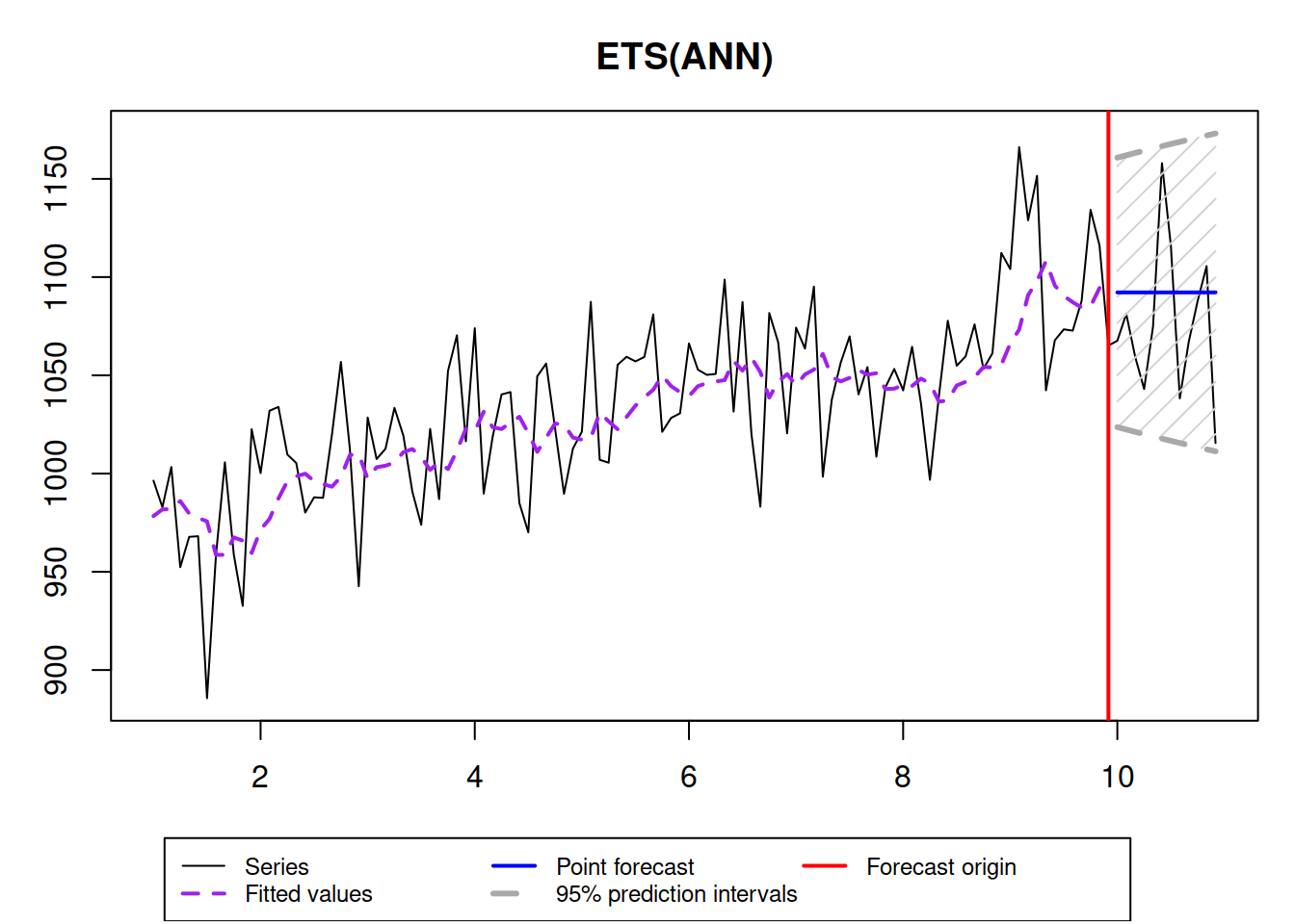
## Time elapsed: 0.03 seconds
## Model estimated: ETS(ANN)
## Persistence vector g:
## alpha
## 0.299
## Initial values were optimised.
##
## Loss function type: likelihood; Loss function value: 510.8823
## Error standard deviation: 27.814
## Sample size: 108
## Number of estimated parameters: 3
## Number of degrees of freedom: 105
## Information criteria:
##      AIC     AICc      BIC     BICc
## 1027.765 1027.995 1035.811 1036.351
##
## 95% parametric prediction interval was constructed
## 92% of values are in the prediction interval
## Forecast errors:
## MPE: -1.3%; sCE: -14.5%; Bias: -47.4%; MAPE: 2.4%
## MASE: 0.795; sMAE: 2.3%; sMSE: 0.1%; rMAE: 0.674; rRMSE: 0.755
As we see, the true smoothing parameter is 0.3, but the estimated one is not exactly 0.3, which is expected, because we deal with an in-sample estimation. Also, notice that with such a high smoothing parameter, the prediction interval is widening with the increase of the forecast horizon. If the smoothing parameter would be lower, then the bounds would not increase, but this might not reflect the uncertainty about the level correctly. Here is an example with \(\alpha=0.01\):
ourModel <- es(y$data, "ANN", h=12, interval=TRUE, holdout=TRUE, silent=FALSE, persistence=0.01)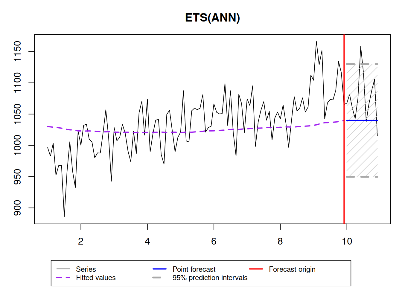 In this case, the prediction interval is wider than needed and the forecast is biased - the model does not keep up to the fast changing time series. So, it is important to correctly estimate the smoothing parameters not only to approximate the data, but also to produce less biased point forecast and more appropriate prediction interval.
5.2.2 ETS(M,N,N)
Hyndman et al. (2008) also demonstrate that there is another ETS model, underlying SES. It is the model with multiplicative error, which is formulated in the following way, as mentioned in a previous chapter: \[\begin{equation} \begin{split} y_{t} &= l_{t-1}(1 + \epsilon_t) \\ l_t &= l_{t-1}(1 + \alpha \epsilon_t) \end{split} , \tag{5.11} \end{equation}\] where \((1+\epsilon_t)\) corresponds to the \(\varepsilon_t\) discussed in the previous section. In order to see the connection of this model with SES, we need to revert to the estimation of the model on the data again: \[\begin{equation} \begin{split} y_{t} &= \hat{l}_{t-1}(1 + e_t) \\ \hat{l}_t &= \hat{l}_{t-1}(1 + \hat{\alpha} e_t) \end{split} , \tag{5.12} \end{equation}\] where \(\hat{y}_t = \hat{l}_{t-1}\) and \(e_t=\frac{y_t - \hat{y}_t}{\hat{y}_t}\). Substituting these values in (5.12) we obtain: \[\begin{equation} \begin{split} y_{t} &= \hat{y}_t (1 + e_t) \\ \hat{y}_{t+1} &= \hat{y}_t \left(1 + \hat{\alpha} \frac{y_t - \hat{y}_t}{\hat{y}_t} \right) \end{split} . \tag{5.13} \end{equation}\] Substituting \(y_t\) with \(\hat{y}_t(1+e_t)\), shifting the indices one step ahead and inserting the second equation to the first one, we get: \[\begin{equation} \hat{y}_{t+1} = \hat{y}_t \left(1 + \hat{\alpha} \frac{y_t - \hat{y}_t}{\hat{y}_t} \right). \tag{5.14} \end{equation}\] Finally, opening the brackets, we get the SES in the form similar to (5.5): \[\begin{equation} \hat{y}_{t+1} = \hat{y}_t + \hat{\alpha} (y_t - \hat{y}_t). \tag{5.15} \end{equation}\]
This example demonstratesonce again the difference between the forecasting method and the forecasting model. When we use SES, we ignore the distributional assumptions, which restricts the usage of the method. The main features of ETS(M,N,N) model in comparison with ETS(A,N,N) are:
- The variance of the actual values in ETS(M,N,N) increases with the increase of the level \(l_{t}\). This allows modelling heteroscedasticity situation in the data;
- If \((1+\epsilon_t)\) is always positive, then the ETS(M,N,N) model will always produce only positive forecasts (both point and interval). This makes this model applicable to the data with low level;
An alternative to (5.11) would be the model (5.6) applied to the data in logarithms (assuming that the data we work with is always positive). However, the ETS(M,N,N) does not rely on exponentiation of the values, making it safe in cases, when very high values are produced by the model (e.g. exp(1000) returns infinity in R).
Finally, the point forecast of ETS(M,N,N) corresponds to the conditional h steps ahead mean and is equal to the last observed level, but only if \(\text{E}(1+\epsilon_t)=1\): \[\begin{equation} \mu_{y,t+h|t} = \hat{y}_{t+h} = l_{t} . \tag{5.16} \end{equation}\]
And here is an example with the ETS(M,N,N) data, which is very similar to the ETS(A,N,N) one:
y <- sim.es("MNN", 120, 1, 12, persistence=0.3, initial=1000)
ourModel <- es(y$data, "MNN", h=12, interval=TRUE, holdout=TRUE, silent=FALSE)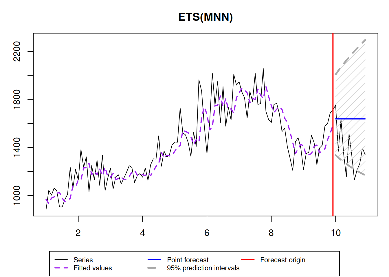
ourModel## Time elapsed: 0.02 seconds
## Model estimated: ETS(MNN)
## Persistence vector g:
## alpha
## 0.3268
## Initial values were optimised.
##
## Loss function type: likelihood; Loss function value: 675.8208
## Error standard deviation: 0.0898
## Sample size: 108
## Number of estimated parameters: 3
## Number of degrees of freedom: 105
## Information criteria:
## AIC AICc BIC BICc
## 1357.642 1357.872 1365.688 1366.228
##
## 95% parametric prediction interval was constructed
## 92% of values are in the prediction interval
## Forecast errors:
## MPE: 3.4%; sCE: 66.2%; Bias: 53.6%; MAPE: 7.1%
## MASE: 1.16; sMAE: 9.7%; sMSE: 1.8%; rMAE: 0.932; rRMSE: 0.947