3.1 Time series components
The main idea behind many forecasting techniques is that any time series can include several unobservable components, such as:
- Level of the series – the average value for a specific time period;
- Growth of the series – the average increase or decrease of the value over a period of time;
- Seasonality – a pattern that repeats itself with a fixed periodicity;
- Error – unexplainable white noise.
Remark. Sometimes, the researchers also include Cycle component, referring to aperiodic long term changes of time series. We do not discuss it here because it is not useful for what follows.
The level is the fundamental component that is present in any time series. In the simplest form (without variability), when plotted on its own without other components, it will look like a straight line, shown, for example, in Figure 3.1.
level <- rep(100,40)
plot(ts(level, frequency=4),
     type="l", xlab="Time", ylab="Sales", ylim=c(80,160))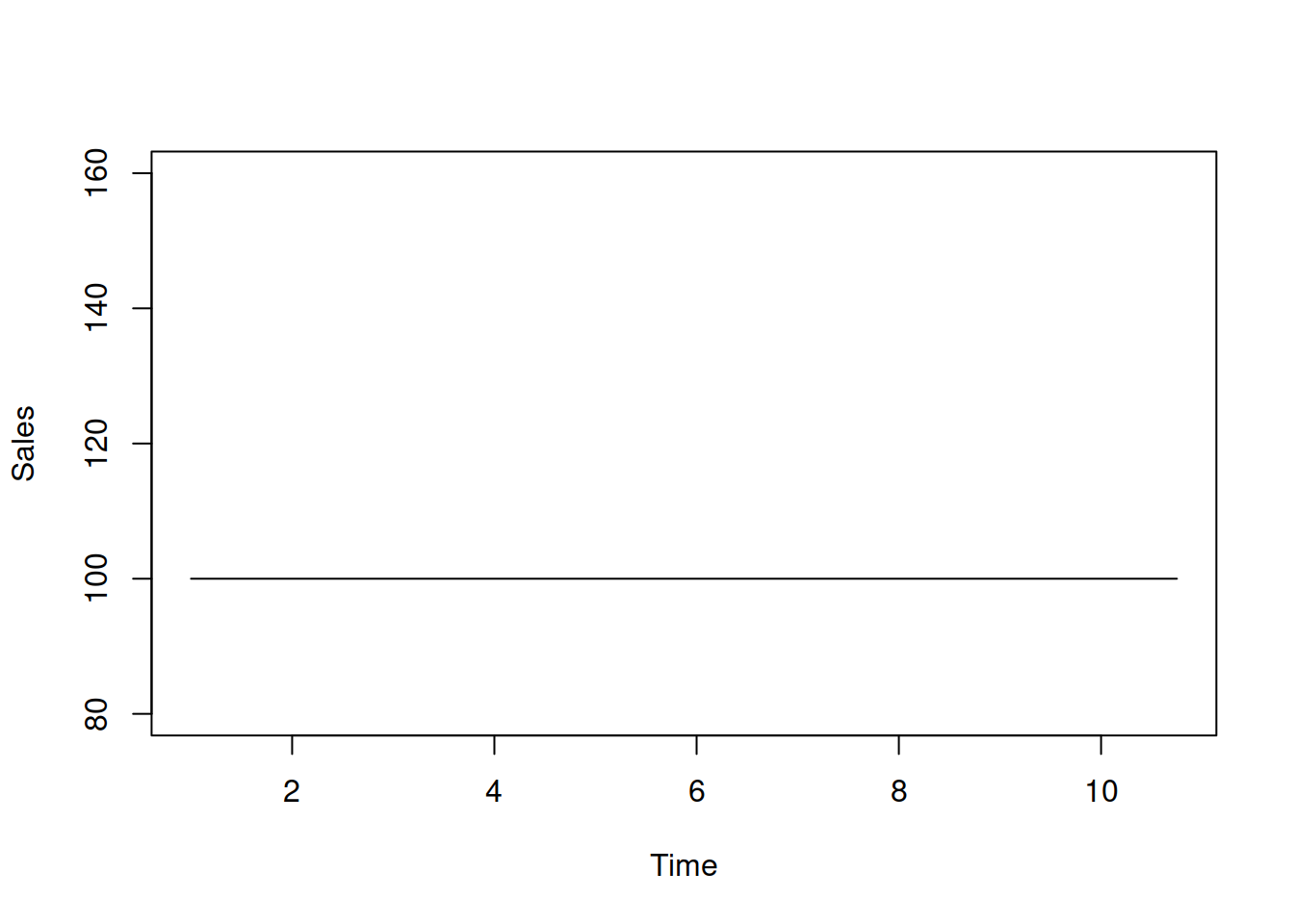
Figure 3.1: Level of time series without any variability.
If the time series exhibits growth, the level will change depending on the observation. For example, if the growth is positive and constant, we can update the level in Figure 3.1 to have a straight line with a non-zero slope as shown in Figure 3.2.
growth <- c(1:40)
plot(ts(level+growth, frequency=4),
     type="l", xlab="Time", ylab="Sales", ylim=c(80,160))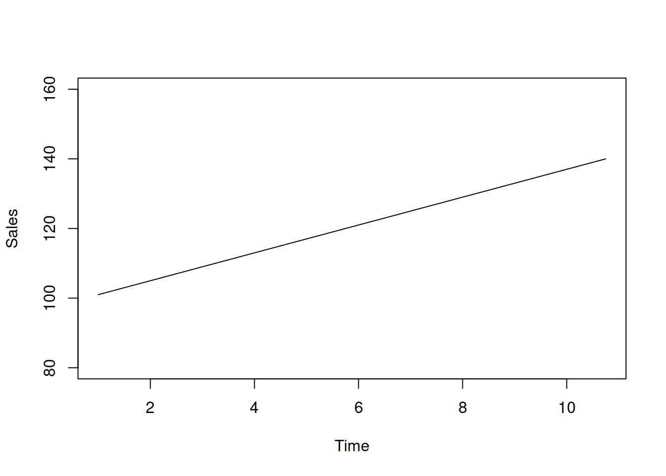
Figure 3.2: Time series with a positive trend and no variability.
The seasonal pattern will introduce some similarities from one period to another. This pattern does not have to literally be seasonal, like beer sales being higher in summer than in winter (seasons of the year). Any pattern with a fixed periodicity works: the number of hospital visitors is higher on Mondays than on Saturdays or Sundays because people tend to stay at home over the weekend. This can be considered as the day of week seasonality. Furthermore, if we deal with hourly data, sales are higher during the daytime than at night (hour of the day seasonality). Adding a deterministic seasonal component to the example above will result in fluctuations around the straight line, as shown in Figure 3.3.
seasonal <- rep(c(10,15,-20,-5),10)
plot(ts(level+growth+seasonal, frequency=4),
     type="l", xlab="Time", ylab="Sales", ylim=c(80,160))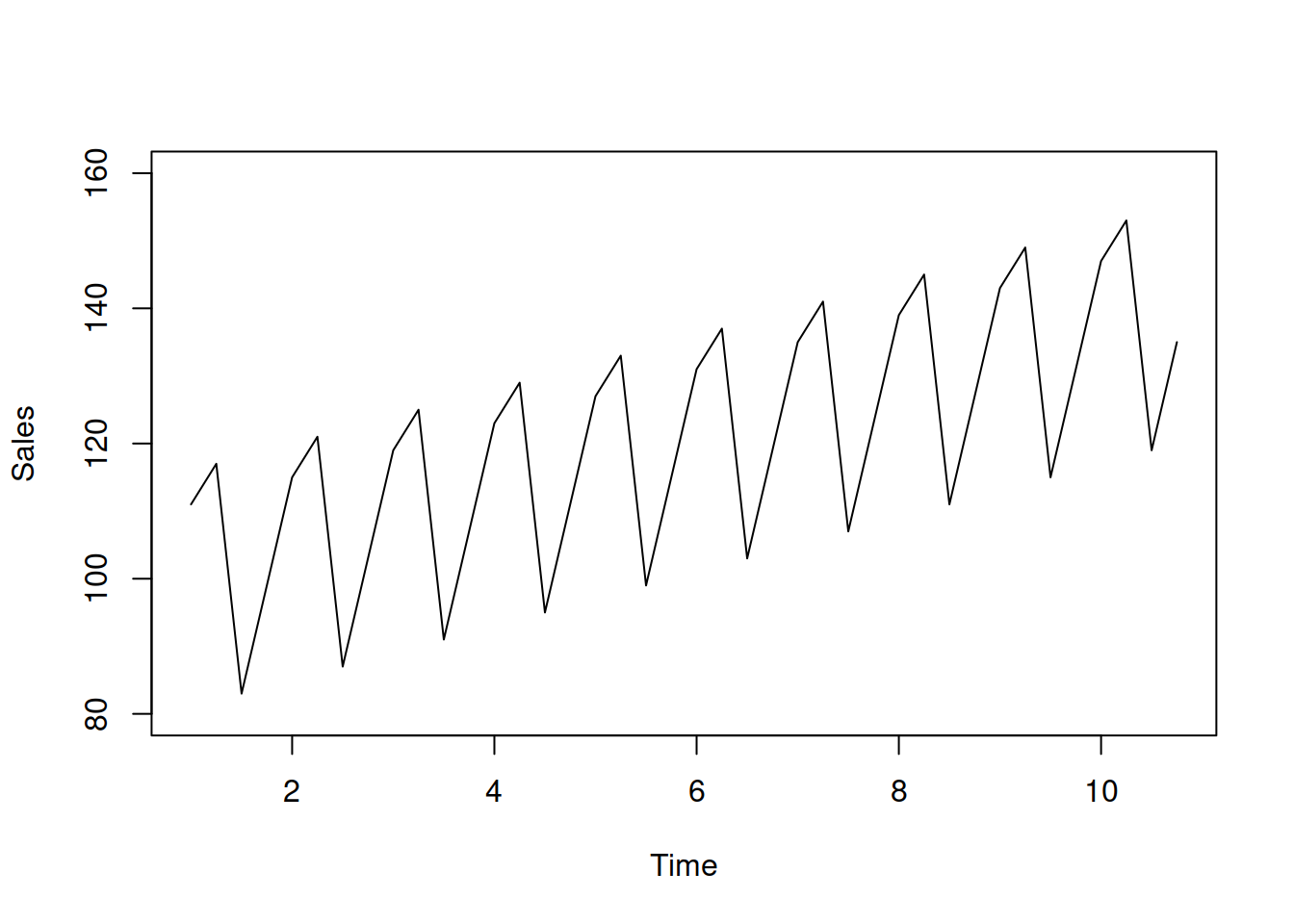
Figure 3.3: Time series with a positive trend, seasonal pattern, and no variability.
Remark. When it comes to giving names to different types of seasonality, you can meet terms like “monthly” and “weekly” or “intra-monthly” and “intra-weekly”. In some cases these names are self explanatory (e.g. when we have monthly data and use the term “monthly” seasonality), but in general this might be misleading. This is why I prefer “frequency 1 of frequency 2” naming, e.g. “month of year” or “week of year”, which is more precise and less ambiguous than the names mentioned above.
Finally, we can introduce the random error to the plots above to have a more realistic time series as shown in Figure 3.4:
par(mfcol=c(3,1),mar=c(2,2,2,1))
error <- rnorm(40,0,5)
plot(ts(level+error, frequency=4),
     type="l", xlab="Time", ylab="Sales", ylim=c(80,160), main="Level time series")
plot(ts(level+growth+error, frequency=4),
     type="l", xlab="Time", ylab="Sales", ylim=c(80,160), main="Time series with growth")
plot(ts(level+growth+seasonal+error, frequency=4),
     type="l", xlab="Time", ylab="Sales", ylim=c(80,160), main="Trend-seasonal time series")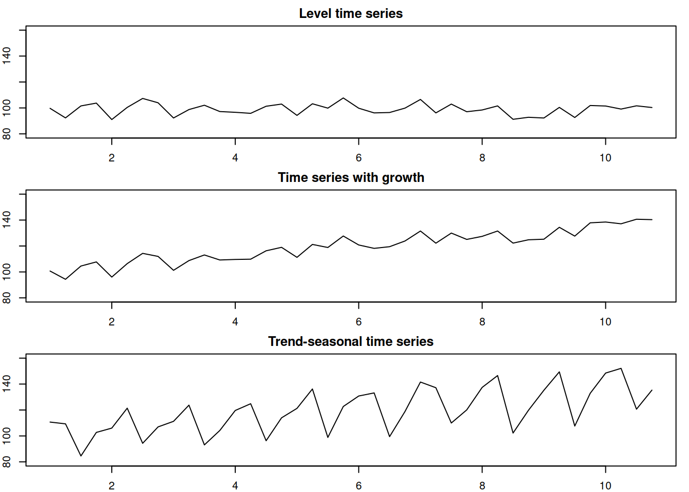
Figure 3.4: Time series with random errors.
Figure 3.4 shows artificial time series with the above components. The level, growth, and seasonal components in those plots are deterministic, they are fixed and do not evolve over time (growth is positive and equal to 1 from year to year). However, in real life, typically, these components will have more complex dynamics, changing over time and thus demonstrating their stochastic nature. For example, in the case of stochastic seasonality, the seasonal shape might change, and instead of having peaks in sales in December, the data would exhibit peaks in February due to the change in consumers’ behaviour.
Remark. Each textbook and paper might use slightly different names to refer to the aforementioned components. For example, in classical decomposition (Persons, 1919), it is assumed that (1) and (2) jointly represent a “trend” component so that a model will contain error, trend, and seasonality.
When it comes to ETS, the growth component (2) is called “trend”, so the model consists of the four components: level, trend, seasonal, and the error term. We will use the ETS formulation in this monograph. According to it, the components can interact in one of two ways: additively or multiplicatively. The pure additive model, in this case, can be written as: \[\begin{equation} y_t = l_{t-1} + b_{t-1} + s_{t-m} + \epsilon_t , \tag{3.1} \end{equation}\] where \(l_{t-1}\) is the level, \(b_{t-1}\) is the trend, \(s_{t-m}\) is the seasonal component with periodicity \(m\) (e.g. 12 for months of year data, implying that something is repeated every 12 months) – all these components are produced on the previous observations and are used on the current one. Finally, \(\epsilon_t\) is the error term, which follows some distribution and has zero mean. The pure additive models were plotted in Figure 3.4. Similarly, the pure multiplicative model is: \[\begin{equation} y_t = l_{t-1} b_{t-1} s_{t-m} \varepsilon_t , \tag{3.2} \end{equation}\] where \(\varepsilon_t\) is the error term with a mean of one. The interpretation of the model (3.1) is that the different components add up to each other, so, for example, the sales increase over time by the value \(b_{t-1}\), and each January they typically change by the amount \(s_{t-m}\), and in addition there is some randomness in the model. The pure additive models can be applied to data with positive, negative, and zero values. In the case of the multiplicative model (3.2), the interpretation is different, showing by how many times the sales change over time and from one season to another. The sales, in this case, will change every January by \((s_{t-m}-1)\)% from the baseline. The model (3.2) only works on strictly positive data (data with purely negative values are also possible but rare in practice).
It is also possible to define mixed models in which, for example, the trend is additive but the other components are multiplicative: \[\begin{equation} y_t = (l_{t-1} + b_{t-1}) s_{t-m} \varepsilon_t \tag{3.3} \end{equation}\] These models work well in practice when the data has large values, far from zero. In other cases, however, they might break and produce strange results (e.g. negative values on positive data), so the conventional decomposition techniques only consider the pure models.
Remark. Sometimes the model with time series components is compared with the regression model. Just to remind the reader, the latter can be formulated as: \[\begin{equation*} {y}_{t} = a_{0} + a_{1} x_{1,t} + a_{2} x_{2,t} + \dots + a_{n} x_{n,t} + \epsilon_t , \end{equation*}\] where \(a_j\) is a \(j\)-th parameter for an explanatory variable \(x_{j,t}\). One of the mistakes that is made in the forecasting context in this case, is to assume that the components resemble explanatory variables in the regression context. This is incorrect. The components correspond to the parameters of a regression model if we allow them to vary over time. We will show in Section 10.5 an example of how the seasonal component \(s_t\) can also be modelled via the parameters of a regression model.