2.1 Measuring accuracy of point forecasts
We start with a setting in which we are interested in point forecasts only. In this case, we typically begin by splitting the available data into training and test sets, applying the models under consideration to the former, and producing forecasts on the latter, hiding it from the models. This is called the “fixed origin” approach: we fix the point in time from which to produce forecasts, produce them, calculate some appropriate error measure, and compare the models.
Different error measures can be used in this case. Which one to use depends on the specific need. Here I briefly discuss the most important measures and refer readers to Davydenko and Fildes (2013), Svetunkov (2019) and Svetunkov (2017) for the gory details.
The majority of point forecast measures rely on the following two popular metrics:
Root Mean Squared Error (RMSE): \[\begin{equation} \mathrm{RMSE} = \sqrt{\frac{1}{h} \sum_{j=1}^h \left( y_{t+j} -\hat{y}_{t+j} \right)^2 }, \tag{2.1} \end{equation}\] and Mean Absolute Error (MAE): \[\begin{equation} \mathrm{MAE} = \frac{1}{h} \sum_{j=1}^h \left| y_{t+j} -\hat{y}_{t+j} \right| , \tag{2.2} \end{equation}\] where \(y_{t+j}\) is the actual value \(j\) steps ahead (values in the test set), \(\hat{y}_{t+j}\) is the \(j\) steps ahead point forecast, and \(h\) is the forecast horizon. As you see, these error measures aggregate the performance of competing forecasting methods across the forecasting horizon, averaging out the specific performances on each \(j\). If this information needs to be retained, the summation can be dropped to obtain “SE” and “AE” values.
In a variety of cases RMSE and MAE might recommend different models, and a logical question would be which of the two to prefer. It is well-known (see, for example, Kolassa, 2016) that the mean value of distribution minimises RMSE, and the median value minimises MAE. So, when selecting between the two, you should consider this property. It also implies, for example, that MAE-based error measures should not be used for the evaluation of models on intermittent demand (see Chapter 13 for the discussion of this topic) because zero forecast will minimise MAE, when the sample contains more than 50% of zeroes (see, for example, Wallström and Segerstedt, 2010).
Another error measure that has been used in some cases is Root Mean Squared Logarithmic Error (RMSLE, see discussion in Tofallis, 2015): \[\begin{equation} \mathrm{RMSLE} = \exp\left(\sqrt{\frac{1}{h} \sum_{j=1}^h \left( \log y_{t+j} -\log \hat{y}_{t+j} \right)^2} \right). \tag{2.3} \end{equation}\] It assumes that the actual values and the forecasts are positive, and it is minimised by the geometric mean. I have added the exponentiation in the formula (2.3), which is sometimes omitted, bringing the metric to the original scale to have the same units as the actual values \(y_t\).
The main difference in the three measures arises when the data we deal with is not symmetric – in that case, the arithmetic, geometric means, and median will all be different. Thus, the error measures might recommend different methods depending on what specifically is produced as a point forecast from the model (see discussion in Section 1.3.1).
Remark. If all your approaches rely on symmetric distributions for the error term (e.g. Normal), the mean and median will coincide. In that case, it becomes unimportant, whether you use MAE or RMSE for forecasts evaluation.
2.1.1 An example in R
In order to see how the error measures work, we consider the following example based on a couple of forecasting functions from the smooth package for R (Hyndman et al., 2008; Svetunkov et al., 2022) and measures from greybox:
# Generate the data
y <- rnorm(100,100,10)
# Apply two models to the data
model1 <- es(y,h=10,holdout=TRUE)
model2 <- ces(y,h=10,holdout=TRUE)
# Calculate RMSE
setNames(sqrt(c(MSE(model1$holdout, model1$forecast),
                MSE(model2$holdout, model2$forecast))),
         c("ETS","CES"))
# Calculate MAE
setNames(c(MAE(model1$holdout, model1$forecast),
           MAE(model2$holdout, model2$forecast)),
         c("ETS","CES"))
# Calculate RMSLE
setNames(exp(sqrt(c(MSE(log(model1$holdout),
                        log(model1$forecast)),
                    MSE(log(model2$holdout),
                        log(model2$forecast))))),
         c("ETS","CES"))
## ETS CES
## 9.492744 9.494683## ETS CES
## 7.678865 7.678846## ETS CES
## 1.095623 1.095626Remark. The point forecasts produced by ETS and CES correspond to conditional means, so ideally we should focus the evaluation on RMSE-based measures.
Given that the distribution of the original data is symmetric, all three error measures should generally recommend the same model. But also, given that the data we generated for the example are stationary, the two models will produce very similar forecasts. The values above demonstrate the latter point – the accuracy between the two models is roughly the same. Note that we have evaluated the same point forecasts from the models using different error measures, which would be wrong if the distribution of the data was skewed. In our case, the model relies on Normal distribution so that the point forecast would coincide with arithmetic mean, geometric mean, and median.
2.1.2 Aggregating error measures
The main advantage of the error measures discussed in the previous subsection is that they are straightforward and have a clear interpretation: they reflect the “average” distances between the point forecasts and the observed values. They are perfect for the work with only one time series. However, they are not suitable when we consider a set of time series, and a forecasting method needs to be selected across all of them. This is because they are scale-dependent and contain specific units: if you measure sales of apples in units, then MAE, RMSE, and RMSLE will show the errors in units as well. And, as we know, you should not add apples to oranges – the result might not make sense.
To tackle this issue, different error scaling techniques have been proposed, resulting in a zoo of error measures:
Remark. Here, I show the principles of scaling, which can be applied to any fundamental measure: MAE, RMSE, RMSLE etc.
- MAPE – Mean Absolute Percentage Error: \[\begin{equation} \mathrm{MAPE} = \frac{1}{h} \sum_{j=1}^h \frac{|y_{t+j} -\hat{y}_{t+j}|}{y_{t+j}}, \tag{2.4} \end{equation}\]
- MASE – Mean Absolute Scaled Error (Hyndman and Koehler, 2006): \[\begin{equation} \mathrm{MASE} = \frac{1}{h} \sum_{j=1}^h \frac{|y_{t+j} -\hat{y}_{t+j}|}{\bar{\Delta}_y}, \tag{2.5} \end{equation}\] where \(\bar{\Delta}_y = \frac{1}{t-1}\sum_{j=2}^t |\Delta y_{j}|\) is the mean absolute value of the first differences \(\Delta y_{j}=y_j-y_{j-1}\) of the in-sample data;
- rMAE – Relative Mean Absolute Error (Davydenko and Fildes, 2013): \[\begin{equation} \mathrm{rMAE} = \frac{\mathrm{MAE}_a}{\mathrm{MAE}_b}, \tag{2.6} \end{equation}\] where \(\mathrm{MAE}_a\) is the mean absolute error of the model under consideration and \(\mathrm{MAE}_b\) is the MAE of the benchmark model;
- sMAE – scaled Mean Absolute Error (Petropoulos and Kourentzes, 2015): \[\begin{equation} \mathrm{sMAE} = \frac{\mathrm{MAE}}{\bar{y}}, \tag{2.7} \end{equation}\] where \(\bar{y}\) is the mean of the in-sample data;
- and others.
Remark. MAPE and sMAE are typically multiplied by 100% to get the percentages, which are easier to work with.
There is no “best” error measure. All have advantages and disadvantages, but some are more suitable in some circumstances than others. For example:
- MAPE is scale sensitive (if the actual values are measured in thousands of units, the resulting error will be much lower than in the case of hundreds of units) and cannot be estimated on data with zeroes. Furthermore, this error measure is biased, preferring when models underforecast the data (see, for example, Makridakis, 1993) and is not minimised by either mean or median, but by an unknown quantity. Accidentally, in the case of Log-Normal distribution, it is minimised by the mode (see discussion in Kolassa, 2016). Despite all the limitations, MAPE has a simple interpretation as it shows the percentage error (as the name suggests);
- MASE avoids the disadvantages of MAPE but does so at the cost of losing a simple interpretation. This is because of the division by the first differences of the data (some interpret this as an in-sample one-step-ahead Naïve forecast, which does not simplify the interpretation);
- rMAE avoids the disadvantages of MAPE, has a simple interpretation (it shows by how much one model is better than the other), but fails, when either \(\mathrm{MAE}_a\) or \(\mathrm{MAE}_b\) for a specific time series is equal to zero. In practice, this happens more often than desired and can be considered a severe error measure limitation. Furthermore, the increase of rMAE (for example, with the increase of sample size) might mean that either the method A is performing better than before or that the method B is performing worse than before – it is not possible to tell the difference unless the denominator in the formula (2.6) is fixed;
- sMAE avoids the disadvantages of MAPE, has an interpretation close to it but breaks down, when the data is non-stationary (e.g. has a trend).
When comparing different forecasting methods, it might make sense to calculate several error measures for comparison. The choice of metric might depend on the specific needs of the forecaster. Here are a few rules of thumb:
- You should typically avoid MAPE and other percentage error measures because the actual values highly influence them in the holdout;
- If you want a robust measure that works consistently, but you do not care about the interpretation, then go with MASE;
- If you want an interpretation, go with rMAE or sMAE. Just keep in mind that if you decide to use rMAE or any other relative measure for research purposes, you might get in an unnecessary dispute with its creator, who might blame you of stealing his creation (even if you reference his work);
- If the data does not exhibit trends (stationary), you can use sMAE.
Furthermore, similarly to the measures above, there have been proposed RMSE-based scaled and relative error metrics, which measure the performance of methods in terms of means rather than medians. Here is a brief list of some of them:
- RMSSE – Root Mean Squared Scaled Error (Makridakis et al., 2022): \[\begin{equation} \mathrm{RMSSE} = \sqrt{\frac{1}{h} \sum_{j=1}^h \frac{(y_{t+j} -\hat{y}_{t+j})^2}{\bar{\Delta}_y^2}} ; \tag{2.8} \end{equation}\]
- rRMSE – Relative Root Mean Squared Error (Stock and Watson, 2004): \[\begin{equation} \mathrm{rRMSE} = \frac{\mathrm{RMSE}_a}{\mathrm{RMSE}_b} ; \tag{2.9} \end{equation}\]
- sRMSE – scaled Root Mean Squared Error (Petropoulos and Kourentzes, 2015): \[\begin{equation} \mathrm{sRMSE} = \frac{\mathrm{RMSE}}{\bar{y}} . \tag{2.10} \end{equation}\]
Similarly, RMSSLE, rRMSLE, and sRMSLE can be proposed, using the same principles as in (2.8), (2.9), and (2.10) to assess performance of models in terms of geometric means across time series.
Finally, when aggregating the performance of forecasting methods across several time series, sometimes it makes sense to look at the distribution of errors – this way, you will know which of the methods fails seriously and which does a consistently good job. If only an aggregate measure is needed then I recommend using both the mean and median of the chosen metric. The mean might be non-finite for some error measures, especially when a method performs exceptionally poorly on a time series (an outlier). Still, it will give you information about the average performance of the method and might flag extreme cases. The median at the same time is robust to outliers and is always calculable, no matter what the distribution of the error term is. Furthermore, comparing mean and median might provide additional information about the tail of distribution without reverting to histograms or the calculation of quantiles. Davydenko and Fildes (2013) argue for the use of geometric mean for relative and scaled measures. Still, as discussed earlier, it might become equal to zero or infinity if the data contains outliers (e.g. two cases, when one of the methods produced a perfect forecast, or the benchmark in rMAE produced a perfect forecast). At the same time, if the distribution of errors in logarithms is symmetric (which is the main argument of Davydenko and Fildes, 2013), then the geometric mean will be similar to the median, so there is no point in calculating the geometric mean at all.
2.1.3 Demonstration in R
In R, there is a variety of functions that calculate the error measures discussed above, including the accuracy() function from the forecast package and measures() from greybox. Here is an example of how the measures can be calculated based on a couple of forecasting functions from the smooth package for R and a set of generated time series:
# Apply a model to a test data to get names of error measures
y <- rnorm(100,100,10)
test <- es(y,h=10,holdout=TRUE)
# Define number of iterations
nsim <- 100
# Create an array for nsim time series,
# 2 models and a set of error measures
errorMeasures <- array(NA, c(nsim,2,length(test$accuracy)),
                       dimnames=list(NULL,c("ETS","CES"),
                                     names(test$accuracy)))
# Start a loop for nsim iterations
for(i in 1:nsim){
  # Generate a time series
  y <- rnorm(100,100,10)
  # Apply ETS
  testModel1 <- es(y,"ANN",h=10,holdout=TRUE)
  errorMeasures[i,1,] <- measures(testModel1$holdout,
                                  testModel1$forecast,
                                  actuals(testModel1))
  # Apply CES
  testModel2 <- ces(y,h=10,holdout=TRUE)
  errorMeasures[i,2,] <- measures(testModel2$holdout,
                                  testModel2$forecast,
                                  actuals(testModel2))
}
The default benchmark method for the relative measures above is Naïve. To see what the distribution of error measures would look like, we can produce violinplots via the vioplot() function from the vioplot package. We will focus on the rRMSE measure (see Figure 2.2).
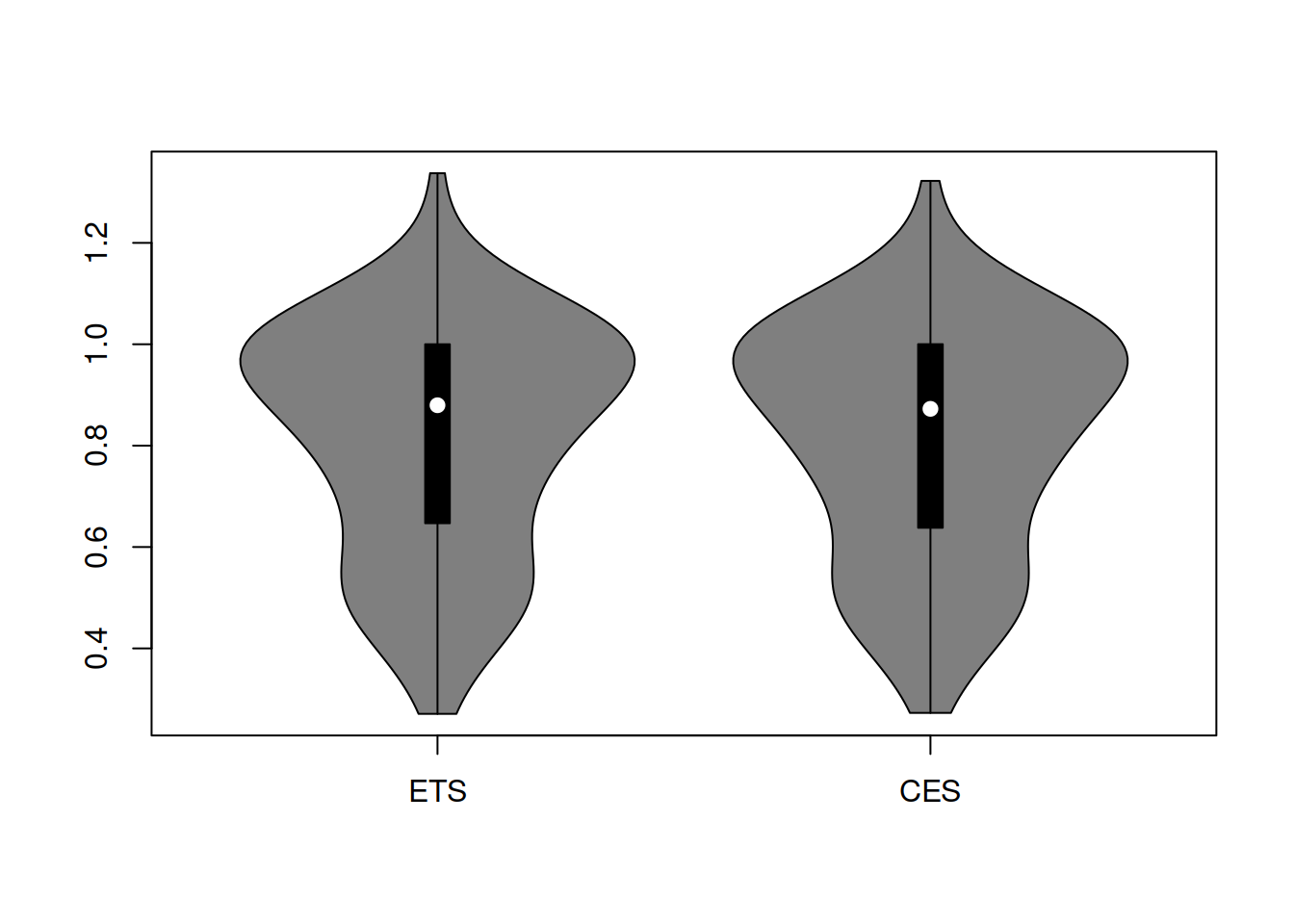
Figure 2.1: Distribution of rRMSE on the original scale.
The distributions in Figure 2.2 look similar, and it is hard to tell which one performs better. Besides, they do not look symmetric, so we will take logarithms to see if this fixes the issue with the skewness (Figure 2.2).
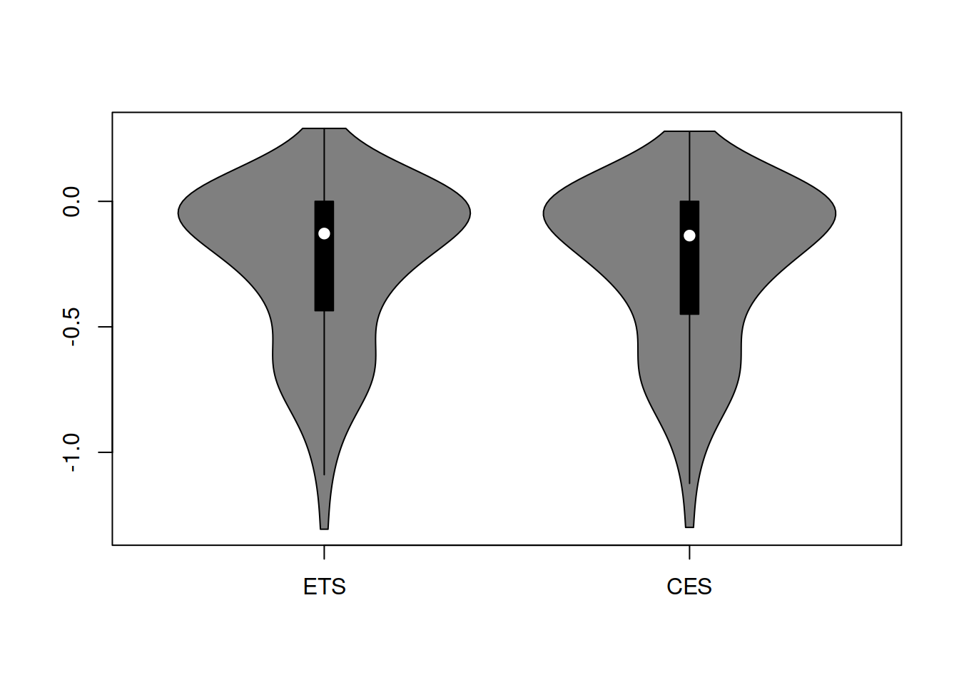
Figure 2.2: Distribution of rRMSE on the log scale.
Figure 2.2 demonstrates that the distribution in logarithms is still skewed, so the geometric mean would not be suitable and might provide a misleading information (being influenced by the tail of distribution). So, we calculate the mean and median rRMSE to check the overall performance of the two models:
##       ETS       CES
## 0.8163452 0.8135303## ETS CES
## 0.8796325 0.8725286Based on the values above, we cannot make any solid conclusion about the performance of the two models; in terms of both mean and median rRMSE, CES is doing slightly better, but the difference between the two models is not substantial, so we can probably choose the one that is easier to work with.