4.1 Model selection mechanism
There are different ways how to select the most appropriate model for the data. One can use judgment, statistical tests, cross-validation or meta learning. The state of the art one in the field of exponential smoothing relies on the calculation of information criteria and on selection of the model with the lowest value. This approach is discussed in detail in Burnham and Anderson (2004). Here we briefly explain how this approach works and what are its advantages and disadvantages.
4.1.1 Information criteria idea
Before we move to the mathematics and well-known formulae, it makes sense to understand what we are trying to do, when we use information criteria. The idea is that we have a pool of model under consideration, and that there is a true model somewhere out there (not necessarily in our pool). This can be presented graphically in the following way:
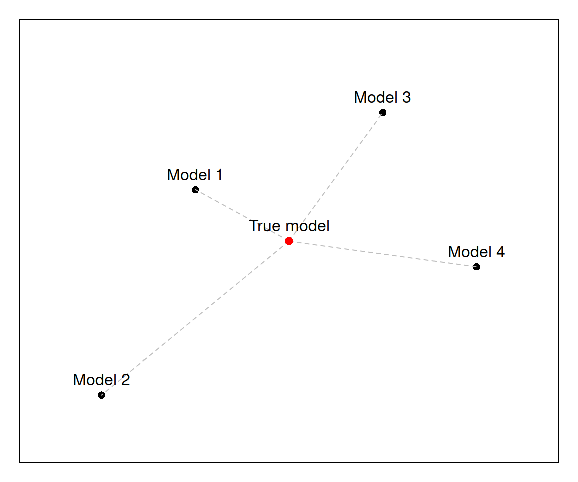
Figure 4.1: An example of a model space
This plot 4.1 represents a space of models. There is a true one in the middle, and there are four models under consideration: Model 1, Model 2, Model 3 and Model 4. They might differ in terms of functional form (additive vs. multiplicative), or in terms of included/omitted variables. All models are at some some distance (the grey dashed lines) from the true model in this hypothetic model space: Model 1 is closest while Model 2 is farthest. Models 3 and 4 have similar distances to the truth.
In the model selection exercise what we typically want to do is to select the model closest to the true one (Model 1 in our case). This is easy to do when you know the true model: just measure the distances and select the closest one. This can be written very roughly as: \[\begin{equation} \begin{split} d_1 = \ell^* - \ell_1 \\ d_2 = \ell^* - \ell_2 \\ d_3 = \ell^* - \ell_3 \\ d_4 = \ell^* - \ell_4 \end{split} , \tag{4.1} \end{equation}\] where \(\ell_j\) is the position of the \(j^{th}\) model and \(\ell^*\) is the position of the true one. One of ways of getting the position of the model is by calculating the log-likelihood (logarithms of likelihood) values for each model, based on the assumed distributions. The likelihood of the true model will always be fixed, so if it is known it just comes to calculating the values for the models 1 - 4, inserting them in the equations in (4.1), and selecting the model that has the lowest distance \(d_j\).
In reality, however, we never know the true model. We therefore need to find some other way of measuring the distances. The neat thing about the maximum likelihood approach is that the true model has the highest possible likelihood by definition! This means that it is not important to know \(\ell^*\) – it will be the same for all the models. So, we can drop the \(\ell^*\) in the formulae (4.1) and compare the models via their likelihoods \(\ell_1, \ell_2, \ell_3 \text{ and } \ell_4\) alone: \[\begin{equation} \begin{split} d_1 = - \ell_1 \\ d_2 = - \ell_2 \\ d_3 = - \ell_3 \\ d_4 = - \ell_4 \end{split} , \tag{4.2} \end{equation}\] This is a very simple method that allows us to get to the model closest to the true one in the pool. However, we should not forget that we usually work with samples of data instead of the entire population and correspondingly will have only estimates of likelihoods and not the true ones. Inevitably, they will be biased and will need to be corrected. Akaike (1974) showed that the bias can be corrected if the number of parameters in each model is added to the distances (4.2) resulting in the bias corrected formula: \[\begin{equation} d_j = k_j - \ell_j \tag{4.3}, \end{equation}\] where \(k_j\) is the number of estimated parameters in model \(j\) (this typically includes scale parameters when dealing with Maximum Likelihood Estimates). Akaike (1974) suggests “An Information Criterion” which multiplies both parts of the right-hand side of (4.3) by 2 so that there is a correspondence between the criterion and the well-known likelihood ratio test (Wikipedia, 2020c): \[\begin{equation} \mathrm{AIC}_j = 2 k_j - 2 \ell_j \tag{4.4}. \end{equation}\]
This criterion now more commonly goes by the “Akaike Information Criterion.”
Various alternative criteria motivated by similar ideas have been proposed. The following are worth mentioning:
AICc (Sugiura, 1978), which is a sample corrected version of the AIC for normal and related distributions, which takes the number of observations into account: \[\begin{equation} \mathrm{AICc}_j = 2 \frac{T}{T-k_j-1} k_j - 2 \ell_j \tag{4.5}, \end{equation}\] where \(T\) is the sample size.
BIC (Schwarz, 1978) (aka “Schwarz criterion”), which is derived from Bayesian statistics: \[\begin{equation} \mathrm{BIC}_j = \log(T) k_j - 2 \ell_j \tag{4.6}. \end{equation}\]
BICc (McQuarrie, 1999) - the sample-corrected version of BIC, relying on the assumption of normality: \[\begin{equation} \mathrm{BICc}_j = \frac{T \log (T)}{T-k_j-1} k_j - 2 \ell_j \tag{4.7}. \end{equation}\]
In general, the use of the sample-corrected versions of the criteria (AICc, BICc) is recommended unless sample size is very large (thousands of observations), in which case the effect of the number of observations on the criteria becomes negligible. The main issue is that corrected versions of information criteria for non-normal distributions need to be derived separately and will differ from (4.5) and (4.7). Still, Burnham and Anderson (2004) recommend using formulae (4.5) and (4.7) in small samples even if the distribution of variables is not normal and the correct formulae are not known. The motivation for this is that the corrected versions still take sample size into account, correcting the sample bias in criteria to some extent.
A thing to note is that the approach relies on asymptotic properties of estimators and assumes that the estimation method used in the process guarantees that the likelihood functions of the models are maximised. In fact, it relies on asymptotic behaviour of parameters, so it is not very important whether the maximum of the likelihood in sample is reached or not or whether the final solution is near the maximum. If the sample size changes, the parameters guaranteeing the maximum will change as well so we cannot get the point correctly in sample anyway. However, it is much more important to use an estimation method that will guarantee consistent maximisation of the likelihood. This implies that we might select wrong models in some cases in sample, but that is okay, because if we use the adequate approach for estimation and selection, with the increase of the sample size, we will select the correct model more often than an incorrect one. While the “increase of sample size” might seem as an unrealistic idea in some real life cases, keep in mind that this might mean not just the increase of \(T\), but also the increase of the number of series under consideration. So, for example, the approach should select the correct model on average, when you test it on a sample of 10,000 SKUs.
Summarising, the idea of model selection via information criteria is to:
- form a pool of competing models,
- construct and estimate them,
- calculate their likelihoods,
- calculate the information criteria,
- and finally, select the model that has the lowest value under the information criterion.
This approach is relatively fast (in comparison with cross-validation, judgmental selection or meta learning) and has good theory behind it. It can also be shown that for normal distributions selecting time series models on the basis of AIC is asymptotically equivalent to the selection based on leave-one-out cross-validation with MSE. This becomes relatively straightforward, if we recall that typically time series models rely on one step ahead errors \((e_t = y_t - \mu_{t|t-1})\) and that the maximum of the likelihood of Normal distribution gives the same estimates as the minimum of MSE.
As for the disadvantages of the approach, as mentioned above, it relies on the in-sample value of the likelihood, based on one step ahead error, and does not guarantee that the selected model will perform well for the holdout for multiple steps ahead. Using the cross-validation or rolling origin for the full horizon could give better results if you suspect that information criteria do not work. Furthermore, any criterion is random on its own, and will change with the sample This means that there is model selection uncertainty and that which model is best might change with new observations. In order to address this issue, combinations of models can be used, which allows mitigating this uncertainty.
4.1.2 Common confusions related to information criteria
Similar to the discussion of hypothesis testing, I have decided to collect common mistakes and confusions related to information criteria. Here they are:
- “AIC relies on Normal distribution.”
- This is not correct. AIC relies on the value of maximised likelihood function. It will use whatever you provide it, so it all comes to the assumptions you make. Having said that, if you use the sample corrected versions of information criteria, such as AICc or BICc, then the formulae (4.5) and (4.7) are derived for Normal distribution. If you use a different one (not related to Normal, so not Log Normal, Box-Cox Normal, Logit Normal etc), then you would need to derive AICc and BICc for it. Still Burnham and Anderson (2004) argue that even if you do not have the correct formula for your distribution, using (4.5) and (4.7) is better than using the non-corrected versions, because there is at least some correction of the bias caused by sample size.
- “We have removed outlier from the model, AIC has decreased.”
- AIC will always decrease if you decrease the sample size and fit the model with the same specification. This is because likelihood function relies on the joint PDF of all observations in sample. If the sample decreases, the likelihood increases. This effect is observed not only in cases, when outliers are removed, but also in case of taking differences of the data. So, when comparing models, make sure that they are constructed on exactly the same data.
- “We have estimated model with logarithm of response variable, and AIC has decreased” (in comparison with the linear one).
- AIC is comparable only between models with the same response variable. If you transform the response variable, you inevitably assume a different distribution. For example, taking logarithm and assuming that error term follows normal distribution is equivalent to assuming that the original data follows log-normal distribution. If you want to make information criteria comparable in this case, either estimate the original model with a different distribution or transform AIC for the multiplicative model.
- “We have used quantile regression, assuming normality and AIC is…”
- Information criteria only work, when the likelihood with the assumed distribution is maximised, because only then it can be guaranteed that the estimates of parameters will be consistent and efficient. If you assume normality, then you either need to maximise the respective likelihood or minimise MSE - they will give the same solution. If you use quantile regression, then you should use likelihood of Asymmetric Laplace. If you estimate parameters via minimisation of MAE, then Laplace distribution of residuals is a suitable assumption for your model. In the cases when distribution and loss are not connected, the selection mechanism might break and not work as intended.