9.5 Examples of application
Building upon the example with AirPassengers data from Section 8.5.2, we will construct several multiplicative ARIMA models and see which one is the most appropriate for the data. As a reminder, the best additive ARIMA model was SARIMA(0,2,2)(1,1,1)\(_{12}\), which had AICc of 1036.075. We will do something similar here, using Log-Normal distribution, thus working with Log-ARIMA. To understand what model can be used in this case, we can take the logarithm of data and see what happens with the components of time series:
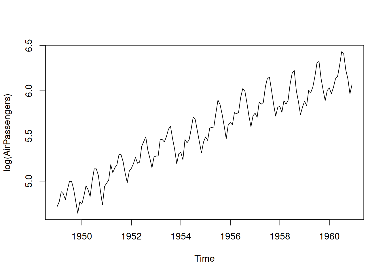
We still have the trend in the data, and the seasonality now corresponds to the additive rather than the multiplicative (as expected). While we might still need the second differences for the non-seasonal part of the model, taking the first differences for the seasonal should suffice because the logarithmic transform will take care of the expanding seasonal pattern in the data. So we can test several models with different options for ARIMA orders:
adamLogSARIMAAir <- vector("list",3)
# logSARIMA(0,1,1)(0,1,1)[12]
adamLogSARIMAAir[[1]] <-
  adam(AirPassengers, "NNN", lags=c(1,12),
       orders=list(ar=c(0,0), i=c(1,1), ma=c(1,1)),
       h=12, holdout=TRUE, distribution="dlnorm")
# logSARIMA(0,2,2)(0,1,1)[12]
adamLogSARIMAAir[[2]] <-
  adam(AirPassengers, "NNN", lags=c(1,12),
       orders=list(ar=c(0,0), i=c(2,1), ma=c(2,2)),
       h=12, holdout=TRUE, distribution="dlnorm")
# logSARIMA(1,1,2)(0,1,1)[12]
adamLogSARIMAAir[[3]] <-
  adam(AirPassengers, "NNN", lags=c(1,12),
       orders=list(ar=c(1,0), i=c(1,1), ma=c(2,1)),
       h=12, holdout=TRUE, distribution="dlnorm")
names(adamLogSARIMAAir) <- c("logSARIMA(0,1,1)(0,1,1)[12]",
                             "logSARIMA(0,2,2)(0,1,1)[12]",
                             "logSARIMA(1,1,2)(0,1,1)[12]")
The thing that is different between the models is the non-seasonal part. Using the connection with ETS (discussed in Section 8.4), the first model should work on local level data, the second should be optimal for the local trend series, and the third one is placed somewhere in between the two. We can compare the models using AICc:
## logSARIMA(0,1,1)(0,1,1)[12] logSARIMA(0,2,2)(0,1,1)[12]
##                    967.7296                   1277.3570
## logSARIMA(1,1,2)(0,1,1)[12]
##                    969.6203
It looks like the logSARIMA(1,1,2)(0,1,1)\(_{12}\) is more appropriate for the data. In order to make sure that we did not miss anything, we analyse the residuals of this model (Figure 9.1):
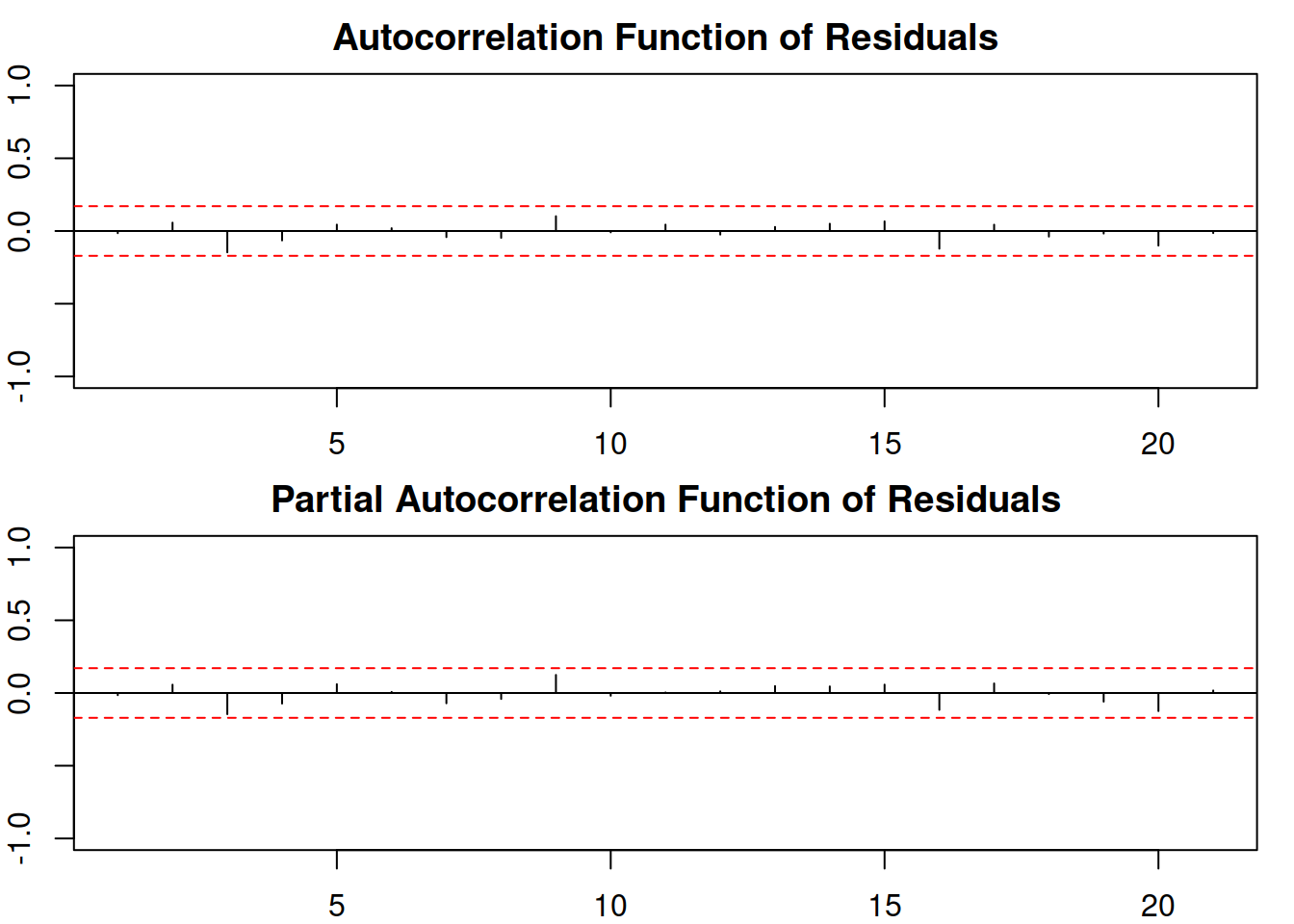
Figure 9.1: ACF and PACF of logSARIMA(1,1,2)(0,1,1)\(_{12}\).
We can see that there are no significant coefficients on either the ACF or PACF, so there is nothing else to improve in this model (we discuss this in more detail in Section 14.5). We can then produce a forecast from the model and see how it performed on the holdout sample (Figure 9.2):
forecast(adamLogSARIMAAir[[3]], h=12, interval="prediction") |>
    plot(main=paste0(adamLogSARIMAAir[[3]]$model,
                     " with Log-Normal distribution"))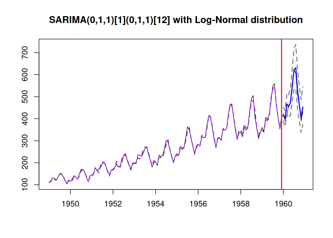
Figure 9.2: Forecast from logSARIMA(1,1,2)(0,1,1)\(_{12}\).
The ETS model closest to the logSARIMA(1,1,2)(0,1,1)\(_{12}\) would probably be ETS(M,M,M), because the former has both seasonal and non-seasonal differences (see discussion in Subsection 8.4.4):
## Time elapsed: 0.04 seconds
## Model estimated using adam() function: ETS(MMM)
## With backcasting initialisation
## Distribution assumed in the model: Gamma
## Loss function type: likelihood; Loss function value: 473.7936
## Persistence vector g:
##  alpha   beta  gamma
## 0.6228 0.0000 0.2300
##
## Sample size: 132
## Number of estimated parameters: 4
## Number of degrees of freedom: 128
## Information criteria:
##      AIC     AICc      BIC     BICc
## 955.5872 955.9021 967.1184 967.8873
##
## Forecast errors:
## ME: -19.086; MAE: 19.377; RMSE: 25.592
## sCE: -87.252%; Asymmetry: -96.4%; sMAE: 7.382%; sMSE: 0.951%
## MASE: 0.805; RMSSE: 0.817; rMAE: 0.255; rRMSE: 0.249
Comparing information criteria, Log-ARIMA should be preferred to ETS(M,M,M). Similar conclusion is achieved if we compare holdout accuracy (based on RMSSE) of the two models:
## Time elapsed: 0.08 seconds
## Model estimated using adam() function: SARIMA(1,1,2)[1](0,1,1)[12]
## With backcasting initialisation
## Distribution assumed in the model: Log-Normal
## Loss function type: likelihood; Loss function value: 479.572
## ARMA parameters of the model:
##         Lag 1
## AR(1) -0.9316
##         Lag 1  Lag 12
## MA(1)  0.7155 -0.4607
## MA(2) -0.2428      NA
##
## Sample size: 132
## Number of estimated parameters: 5
## Number of degrees of freedom: 127
## Information criteria:
##      AIC     AICc      BIC     BICc
## 969.1441 969.6203 983.5581 984.7206
##
## Forecast errors:
## ME: -15.106; MAE: 15.955; RMSE: 20.776
## sCE: -69.058%; Asymmetry: -93.1%; sMAE: 6.078%; sMSE: 0.626%
## MASE: 0.662; RMSSE: 0.663; rMAE: 0.21; rRMSE: 0.202
To get a better idea about the holdout performance of the two models, we would need to apply them in the rolling origin fashion (Section 2.4), collect a distribution of errors, and then decide, which one to choose.