7.4 Mixed models with multiplicative trend
This is the most challenging class of models (MMA; MMdA; AMN; AMdN; AMA; AMdA; AMM; AMdM). They do not have analytical formulae for conditional moments, and they are very sensitive to smoothing parameter values and may lead to explosive forecasting trajectories. So, to obtain the conditional expectation, variance, and prediction interval from the models of these classes, simulations should be used.
One of the issues encountered when using these models is the explosive trajectories because of the multiplicative trend. As a result, when these models are estimated, it makes sense to set the initial value of the trend to 1 or a lower value so that the optimiser does not encounter difficulties in the calculations because of the explosive behaviour in-sample.
Furthermore, the combinations of components for the models in this class make even less sense than the combinations for Class C (discussed in Section 7.3). For example, the multiplicative trend assumes either explosive growth or decay, as shown in Figure 7.1.
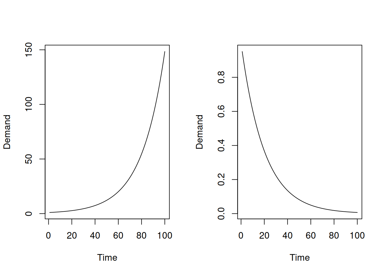
Figure 7.1: Plots of exponential increase and exponential decline.
However, assuming that either the seasonal component, the error term, or both will have precisely the same impact on the final value irrespective of the point of time (thus being additive) is unrealistic for this situation. The more reasonable one would be for the amplitude of seasonality to decrease together with the exponential decay of the trend and for the variance of the error term to do the same. But this means that we are talking about the pure multiplicative models (Chapter 6.1), not the mixed ones. There is only one situation where such mixed models could make sense: when the speed of change of the exponential trajectory is close to zero (i.e. the trend behaves similar to the linear one) and when the volume of the data is high. In this case, the mixed models might perform well and even produce more accurate forecasts than the models from the other classes.
When it comes to the bounds of the parameters, this is a mystery for the mixed models of this class. This is because the recursive relations are complicated, and calculating the discount matrix or anything like that becomes challenging. The usual bounds should still be okay, but keep in mind that these mixed models are typically not very stable and might exhibit explosive behaviour even, for example, with \(\beta=0.1\). So from my experience, the smoothing parameters in these models should be as low as possible, assuming that the initial values guarantee a working model (not breaking on some of the observations).