14.8 Residuals are i.i.d.: Distributional assumptions
Finally, we come to the distributional assumptions of ADAM. If we use a wrong distribution then we might get incorrect estimates of parameters and we might end up with miscallibrated prediction intervals (i.e. quantiles from the model will differ from the theoretical ones substantially).
As discussed earlier (for example, in Section 11.1), the ADAM framework supports several distributions. The specific parts of assumptions will change depending on the type of error term in the model. Given that, it is relatively straightforward to see if the residuals of the model follow the assumed distribution or not, and there exist several tools for that.
The simplest one is called a Quantile-Quantile (QQ) plot. It produces a figure with theoretical vs actual quantiles and shows whether they are close to each other or not. Here is, for example, how the QQ plot will look for one of the previous models, assuming Normal distribution (Figure 14.27):
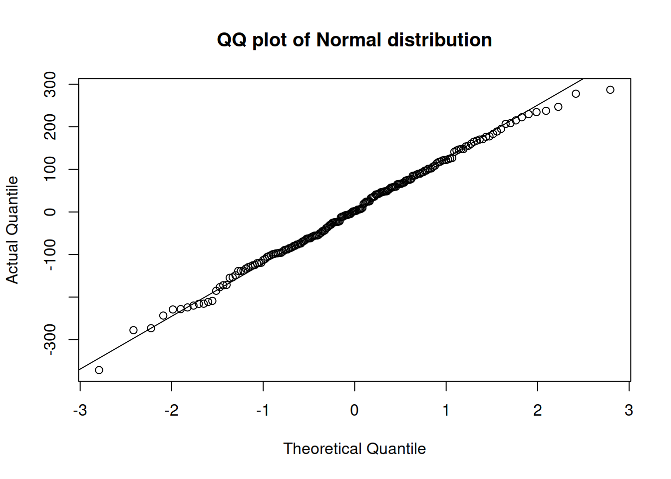
Figure 14.27: QQ plot of residuals extracted from model 3.
If the residuals do not contradict the assumed distribution, all the points should lie either very close to or on the line. In our case, in Figure 14.27, most points are close to the line, but the tails (especially the right one) are slightly off. This might mean that we should either use a different error type or a different distribution. Just for the sake of argument, we can try an ETSX(M,N,M) model, with the same set of explanatory variables as in the model adamSeat03, and with the same Normal distribution:
adamSeat16 <- adam(Seatbelts, "MNM",
                   formula=drivers~log(PetrolPrice)+log(kms)+law,
                   distribution="dnorm")
plot(adamSeat16, which=6)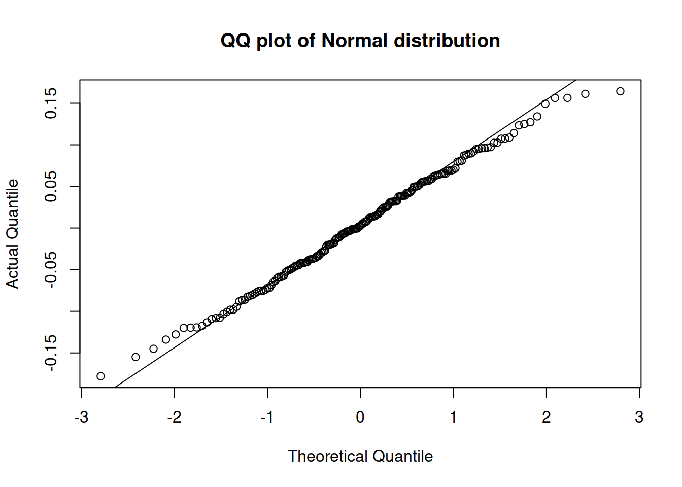
Figure 14.28: QQ plot of residuals extracted from the multiplicative model with Normal distribution.
According to the QQ plot in Figure 14.28, the residuals of the new model are still not very close to the theoretical ones. The tails have a slight deviation from normality: both of them are slightly shorter than expected. If our aim is to capture the distribution correctly then this can be addressed by using a Generalised Normal distribution with a higher shape parameter, which will have lighter tails. Hopefully, ADAM can estimate the shape parameters correctly in our case:
adamSeat17 <- adam(Seatbelts, "MNM",
                   formula=drivers~log(PetrolPrice)+log(kms)+law,
                   distribution="dgnorm")
plot(adamSeat17, which=6)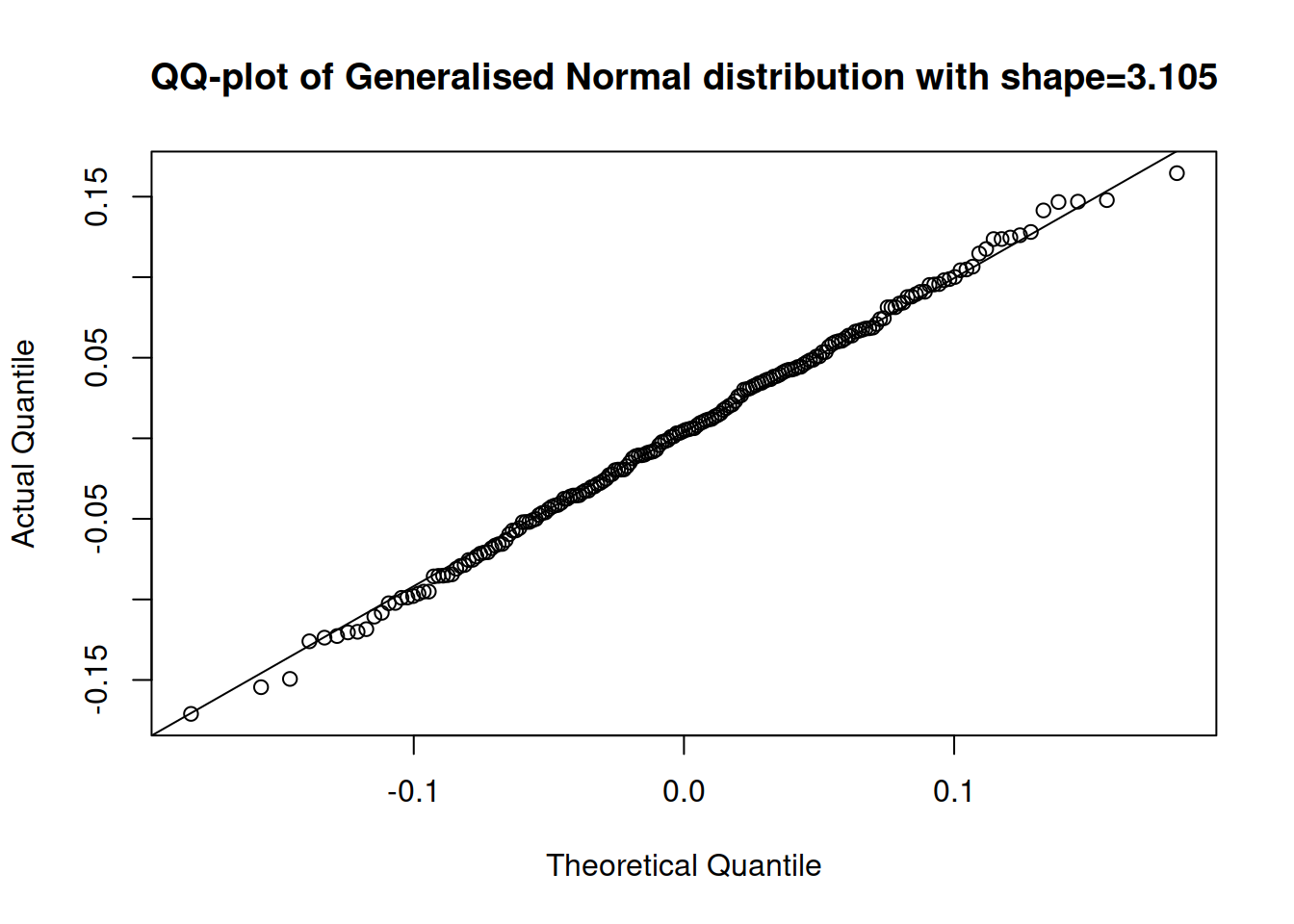
Figure 14.29: QQ plot of residuals extracted from the multiplicative model with Gamma distribution.
The QQ plot in Figure 14.29 shows that the residuals of Model 17 are closer to the parametric distribution than in the cases of the two previous models. We could use AICc to select between the two models if we are not sure, which of them to prefer:
## [1] 2385.686## [1] 2386.382Based on these results, we can conclude that the model with the Generalised Normal distribution is more suitable for this situation than the one assuming Normality.
Another way to analyse the distribution of residuals is to plot a histogram together with the theoretical probability density function (PDF). Here is an example for Model 3:
# Plot histogram of residuals
hist(residuals(adamSeat03), probability=TRUE,
     xlab="Residuals", main="", ylim=c(0,0.0035))
# Add density line of the theoretical distribution
lines(seq(-400,400,1),
      dnorm(seq(-400,400,1),
            mean(residuals(adamSeat03)),
            adamSeat03$scale),
      col="red")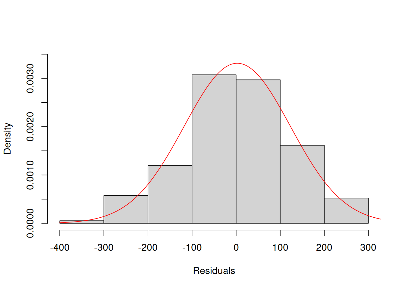
Figure 14.30: Histogram and density line for the residuals from Model 3 (assumed to follow Normal distribution).
However, the plot in Figure 14.30 is arguably more challenging to analyse than the QQ plot – it is not clear whether the distribution is close to the theoretical one or not. For example, Figure 14.31 shows how the histogram and the PDF curve would look for Model 17 which had the best distributional fit (assuming Generalised Normal distribution).
# Plot histogram of residuals
hist(residuals(adamSeat17), probability=TRUE,
     xlab="Residuals", main="")
# Add density line of the theoretical distribution
lines(seq(-0.2,0.2,0.01),
      dgnorm(seq(-0.2,0.2,0.01), mean(residuals(adamSeat17)),
             adamSeat17$scale, adamSeat17$other$shape),
      col="red")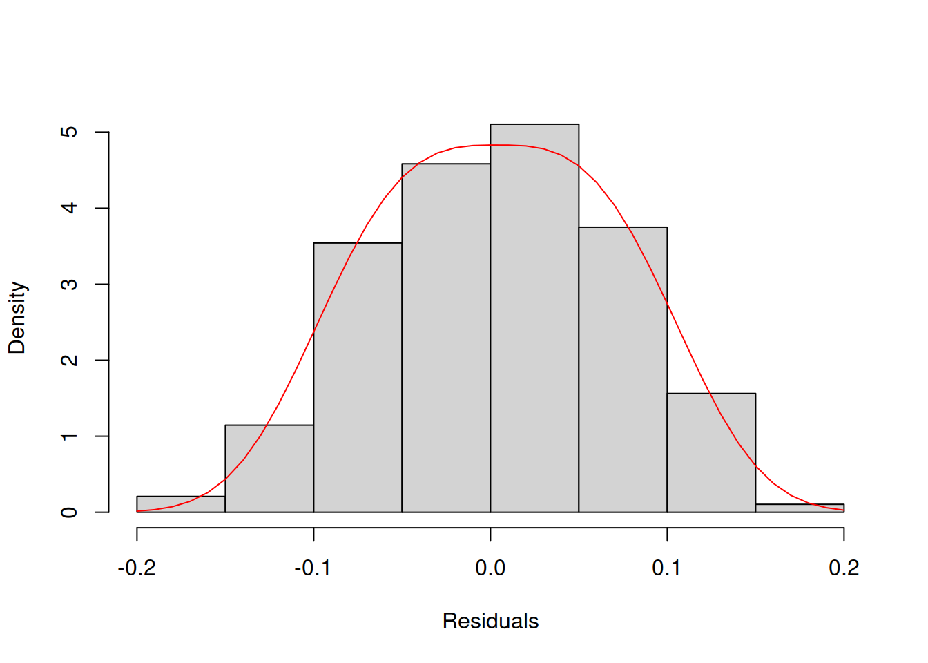
Figure 14.31: Histogram and density line for the residuals from model 17 (assumed to follow Generalised Normal distribution).
Comparing the plots in Figures 14.30 and 14.31 is a challenging task. This is why in general, I would recommend using QQ plots instead of histograms.
There are also formal tests for the distribution of residuals, such as Shapiro-Wilk (Shapiro and Wilk, 1965), Anderson-Darling (Anderson and Darling, 1952), and others. However, I prefer to use visual inspection when possible instead of these tests because, as discussed in Section 7.1 of Svetunkov and Yusupova (2025), the null hypothesis is always wrong whatever the test you use. In practice, it will inevitably be rejected with the increase of the sample size, which does not mean that it is either correct or wrong. Besides, if you fail to reject H\(_0\), it does not mean that your variable follows the assumed distribution. It only means that you have not found enough evidence to reject the null hypothesis.