8.1 Introduction to ARIMA
ARIMA contains several elements:
- AR(p) – the AutoRegressive part, showing how the variable is impacted by its values on the previous observations. It contains \(p\) lags. For example, the quantity of the liquid in a vessel with an opened tap on some observation will depend on the quantity on the previous steps;
- I(d) – the number of differences \(d\) taken in the model (I stands for “Integrated”). Working with differences rather than with the original data means that we deal with changes and rates of changes, rather than the original values. Technically, differences are needed to make data stationary (i.e. with fixed expectation and variance, although there are different definitions of the term stationarity, see below);
- MA(q) – the Moving Average component, explaining how the previous white noise impacts the variable. It contains \(q\) lags. Once again, in technical systems, the idea that random error can affect the value has a relatively simple explanation. For example, when the liquid drips out of a vessel, we might not be able to predict the air fluctuations, which would impact the flow and could be perceived as elements of random noise. This randomness might, in turn, influence the quantity of liquid in a vessel on the following observation, thus introducing the MA elements in the model.
I intentionally do not provide ARIMA examples from the demand forecasting area, as these are much more difficult to motivate and explain than the examples from the more technical areas.
Before continuing our discussion, we should define the term stationarity. There are two definitions in the literature: one refers to “strict stationarity”, while the other refers to the “weak stationarity”:
- Time series is said to be weak stationary when its unconditional expectation and variance are constant, and the variance is finite on all observations;
- Time series is said to be strong stationary when its unconditional joint probability distribution does not change over time. This automatically implies that all its moments are constant (i.e. the process is also weak stationary).
The stationarity is essential in the ARIMA context and plays an important role in regression analysis. If the series is not stationary, it might be challenging to estimate its moments correctly using conventional methods. In some cases, it might be impossible to get the correct parameters (e.g. there is an infinite combination of parameters that would produce the minimum of the selected loss function). To avoid this issue, the series is transformed to ensure that the moments are finite and constant. Taking differences or detrending time series (e.g. via seasonal decomposition discussed in Section 3.2) allows making the first moment (mean) constant, while taking logarithms or doing the Box-Cox transform of the original series typically stabilises the variance, making it constant as well. After that, the model becomes easier to identify.
In contrast with ARIMA, the ETS models are almost always non-stationary and do not require the series to be stationary. We will see the connection between the two approaches in Section 8.4.
Finally, conventional ARIMA is always a pure additive model, and as a result its point forecasts coincide with the conditional expectation, and it has closed forms for the conditional moments and quantiles.
8.1.1 AR(p)
We start with a simple AR(1) model, which is written as: \[\begin{equation} {y}_{t} = \phi_1 y_{t-1} + \epsilon_t , \tag{8.1} \end{equation}\] where \(\phi_1\) is the parameter of the model. This formula tells us that the value on the previous observation is carried over to the new one in the proportion of \(\phi_1\). Typically, the parameter \(\phi_1\) is restricted with the region (-1, 1) to make the model stationary, but very often in real life, \(\phi_1\) lies in the (0, 1) region. If the parameter is equal to one, the model becomes equivalent to Random Walk (Section 3.3.1).
The forecast trajectory (conditional expectation several steps ahead) of this model would typically correspond to the exponentially declining curve. This is because for the \(y_{t+h}\) value, AR(1) is: \[\begin{equation} {y}_{t+h} = \phi_1 y_{t+h-1} + \epsilon_{t+h} = \phi_1^2 y_{t+h-2} + \phi_1 \epsilon_{t+h-1} + \epsilon_{t+h} = \dots \phi_1^h y_{t} + \sum_{j=0}^{h-1} \phi_1^{j} \epsilon_{t+h-j}. \tag{8.2} \end{equation}\] If we then take expectation conditional on the information available up until observation \(t\), all error terms will disappear (because we assume that \(\mathrm{E}(\epsilon_{t+j})=0\) for all \(j\)) leading to: \[\begin{equation} \mathrm{E}({y}_{t+h} |t) = \phi_1^h y_{t} . \tag{8.3} \end{equation}\] If \(\phi_1 \in (0, 1)\), the forecast trajectory will decline exponentially.
Here is a simple example in R of a very basic forecast from AR(1) with \(\phi_1=0.9\) (see Figure 8.1):
y <- vector("numeric", 20)
y[1] <- 100
phi <- 0.9
for(i in 2:length(y)){
    y[i] <- phi * y[i-1]
}
plot(y, type="l", xlab="Horizon", ylab="Forecast")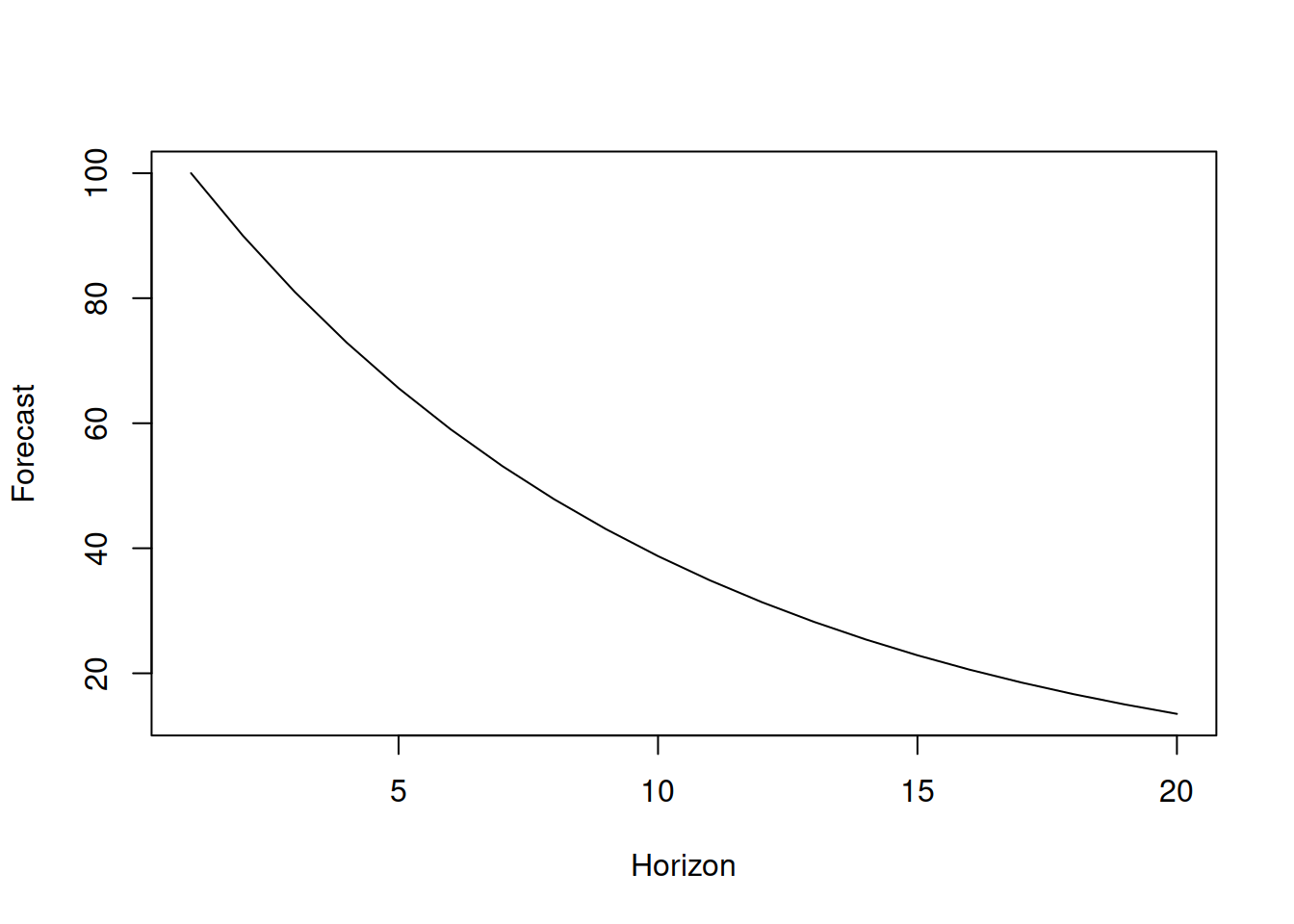
Figure 8.1: Forecast trajectory for AR(1) with \(\phi_1=0.9\).
If, for some reason, we get \(\phi_1>1\), then the trajectory will exhibit an exponential increase, becoming explosive, implying non-stationary behaviour. The model, in this case, becomes very difficult to work with, even if the parameter is close to one. So it is typically advised to restrict the parameter with the stationarity region (we will discuss this in more detail later in this chapter).
In general, it is possible to imagine the situation, when the value at the moment of time \(t\) would depend on several previous values, so the model AR(p) would be needed: \[\begin{equation} {y}_{t} = \phi_1 y_{t-1} + \phi_2 y_{t-2} + \dots + \phi_p y_{t-p} + \epsilon_t , \tag{8.4} \end{equation}\] where \(\phi_i\) is the parameter for the \(i\)-th lag of the model. So, the model assumes that the data on the recent observation is influenced by the \(p\) previous observations. The more lags we introduce in the model, the more complicated the forecasting trajectory becomes, potentially demonstrating harmonic behaviour. Here is an example of a point forecast from an AR(3) model \({y}_{t} = 0.9 y_{t-1} -0.7 y_{t-2} + 0.6 y_{t-3} + \epsilon_t\) (Figure 8.2):
y <- vector("numeric", 30)
y[1:3] <- c(100, 75, 30)
phi <- c(0.9,-0.7,0.6)
for(i in 4:30){
    y[i] <- phi[1] * y[i-1] + phi[2] * y[i-2] + phi[3] * y[i-3]
}
plot(y, type="l", xlab="Horizon", ylab="Forecast")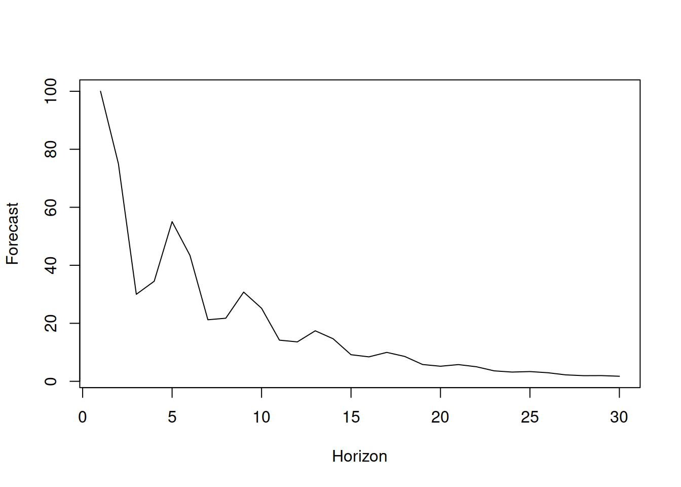
Figure 8.2: Forecast trajectory for an AR(3) model.
No matter what the forecast trajectory of the AR model is, it will asymptotically converge to zero as long as the model is stationary.
An example of an AR(3) time series generated using the sim.ssarima() function from the smooth package and a forecast for it via msarima() is shown in Figure 8.3.
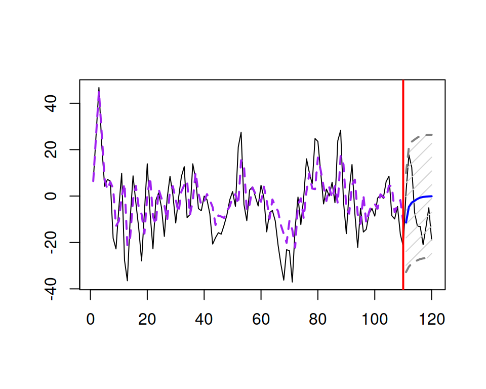
Figure 8.3: An example of an AR(3) series and a forecast for it.
As can be seen from Figure 8.3, the series does not exhibit any distinct characteristics so that it would be possible to identify the order of the model just by looking at it. The only thing that we can probably say is that there is some structure in it: it has some periodic fluctuations and some parts of series are consistently above zero, while the others are consistently below. The latter is an indicator of autocorrelation in data. We do not discuss how to identify the order of AR in this section, but we will come back to it in Section 8.3.
8.1.2 MA(q)
Before discussing the “Moving Averages” model, we should acknowledge that the name is quite misleading and that the model has nothing to do with Centred Moving Averages used in time series decomposition (Section 3.2) or Simple Moving Averages (discussed in Section 3.3.3) used in forecasting. The idea of the simplest MA(1) model can be summarised in the following mathematical way: \[\begin{equation} {y}_{t} = \theta_1 \epsilon_{t-1} + \epsilon_t , \tag{8.5} \end{equation}\] where \(\theta_1\) is the parameter of the model, typically lying between (-1, 1), showing what part of the error is carried out to the next observation. Because of the conventional assumption that the error term has a zero mean (\(\mathrm{E}(\epsilon_{t})=0\)), the forecast trajectory of this model is just a straight line coinciding with zero starting from the \(h=2\). But for the one step ahead point forecast we have: \[\begin{equation} \mathrm{E}({y}_{t+1}|t) = \theta_1 \mathrm{E}(\epsilon_{t}|t) + \mathrm{E}(\epsilon_{t+1}|t) = \theta_1 \epsilon_{t}. \tag{8.6} \end{equation}\] Starting from \(h=2\) there are no observable error terms \(\epsilon_t\), so all the values past that are equal to zero: \[\begin{equation} \mathrm{E}({y}_{t+2}|t) = \theta_1 \mathrm{E}(\epsilon_{t+1}|t) + \mathrm{E}(\epsilon_{t+2}|t) = 0. \tag{8.7} \end{equation}\] So, the forecast trajectory for the MA(1) model drops to zero, when \(h>1\).
More generally, the MA(q) model is written as: \[\begin{equation} {y}_{t} = \theta_1 \epsilon_{t-1} + \theta_2 \epsilon_{t-2} + \dots + \theta_q \epsilon_{t-q} + \epsilon_t , \tag{8.8} \end{equation}\] where \(\theta_i\) is the parameters for the \(i\)-th lag of the error term, typically restricted with the so-called invertibility region (discussed in the next section). In this case, the model implies that the recent observation is influenced by several errors on previous observations (your mistakes in the past will haunt you in the future). The more lags we introduce, the more complicated the model becomes. As for the forecast trajectory, it will reach zero when \(h>q\).
An example of an MA(3) time series and a forecast for it is shown in Figure 8.4.
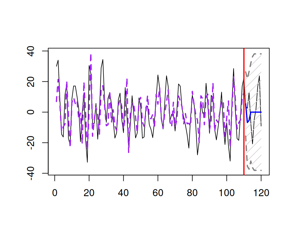
Figure 8.4: An example of an MA(3) series and forecast for it.
Similarly to how it was with AR(3), Figure 8.4 does not show anything specific that could tell us that this is an MA(3) process. The proper identification of MA orders will be discussed in Section 8.3.
8.1.3 ARMA(p,q)
Connecting the models (8.4) and (8.8), we get the more complicated model, ARMA(p,q): \[\begin{equation} {y}_{t} = \phi_1 y_{t-1} + \phi_2 y_{t-2} + \dots + \phi_p y_{t-p} + \theta_1 \epsilon_{t-1} + \theta_2 \epsilon_{t-2} + \dots + \theta_q \epsilon_{t-q} + \epsilon_t , \tag{8.9} \end{equation}\] which has the properties of the two models discussed above. The forecast trajectory from this model will have a combination of trajectories for AR and MA for \(h \leq q\) and then will correspond to AR(p) for \(h>q\).
To simplify the work with ARMA models, the equation (8.9) is typically rewritten by moving all terms with \(y_t\) to the left-hand side: \[\begin{equation} {y}_{t} -\phi_1 y_{t-1} -\phi_2 y_{t-2} -\dots -\phi_p y_{t-p} = \epsilon_t + \theta_1 \epsilon_{t-1} + \theta_2 \epsilon_{t-2} + \dots + \theta_q \epsilon_{t-q} . \tag{8.10} \end{equation}\] Furthermore, in order to make this even more compact, the backshift operator B can be introduced. It just shows by how much the subscript of the variable is shifted back in time: \[\begin{equation} {y}_{t} B^i = {y}_{t-i}. \tag{8.11} \end{equation}\] Using (8.11), the ARMA model can be written as: \[\begin{equation} {y}_{t} (1 -\phi_1 B -\phi_2 B^2 -\dots -\phi_p B^p) = \epsilon_t (1 + \theta_1 B + \theta_2 B^2 + \dots + \theta_q B^q) . \tag{8.12} \end{equation}\] Finally, we can also introduce the AR and MA polynomial functions (corresponding to the elements in the brackets of (8.12)) to make the model even more compact: \[\begin{equation} \begin{aligned} & \varphi^p(B) = 1 -\phi_1 B -\phi_2 B^2 -\dots -\phi_p B^p \\ & \vartheta^q(B) = 1 + \theta_1 B + \theta_2 B^2 + \dots + \theta_q B^q . \end{aligned} \tag{8.13} \end{equation}\] Inserting the functions (8.13) in (8.12) leads to the compact presentation of the ARMA model: \[\begin{equation} {y}_{t} \varphi^p(B) = \epsilon_t \vartheta^q(B) . \tag{8.14} \end{equation}\] The model (8.14) can be considered a compact form of (8.9). It is more difficult to understand and interpret but easier to work with from a mathematical point of view. In addition, this form permits introducing additional elements, which will be discussed later in this chapter.
Figure 8.5 shows an example of an ARMA(3,3) series with a forecast from it.
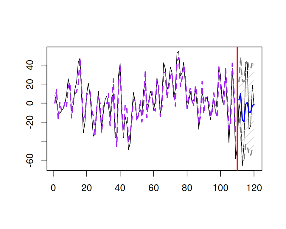
Figure 8.5: An example of an ARMA(3,3) series and a forecast for it.
Similarly to the AR(3) and MA(3) examples above, the process is not visually distinguishable from other ARMA processes.
Coming back to the ARMA model (8.9), as discussed earlier, it assumes convergence of forecast trajectory to zero, the speed of which is regulated by its parameters. This implies that the data has the mean of zero, and ARMA should be applied to somehow pre-processed data so that it is stationary and varies around zero. This means that if you work with non-stationary and/or with non-zero mean data, the pure AR/MA or ARMA will be inappropriate – some prior transformations will be required.
8.1.4 ARMA with constant
One of the simpler ways to deal with the issue with zero forecasts is to introduce the constant (or intercept) in ARMA: \[\begin{equation} {y}_{t} = a_0 + \phi_1 y_{t-1} + \phi_2 y_{t-2} + \dots + \phi_p y_{t-p} + \theta_1 \epsilon_{t-1} + \theta_2 \epsilon_{t-2} + \dots + \theta_p \epsilon_{t-p} + \epsilon_t \tag{8.15} \end{equation}\] or \[\begin{equation} {y}_{t} \varphi^p(B) = a_0 + \epsilon_t \vartheta^q(B) , \tag{8.16} \end{equation}\] where \(a_0\) is the constant parameter, which in this case also works as the unconditional mean of the series. The forecast trajectory in this case would converge to a non-zero number, but with some minor differences from the trajectory of ARMA without constant. For example, in case of ARMA(1,1) with constant we will have: \[\begin{equation} {y}_{t} = a_0 + \phi_1 y_{t-1} + \theta_1 \epsilon_{t-1} + \epsilon_t . \tag{8.17} \end{equation}\] The conditional expectation of \(y_{t+h}\) for \(h=1\) and \(h=2\) can be written as (based on the discussions in previous sections): \[\begin{equation} \begin{aligned} & \mathrm{E}({y}_{t+1}|t) = a_0 + \phi_1 y_{t} + \theta_1 \epsilon_{t} \\ & \mathrm{E}({y}_{t+2}|t) = a_0 + \phi_1 \mathrm{E}(y_{t+1}|t) = a_0 + \phi_1 a_0 + \phi_1^2 y_{t} + \phi_1 \theta_1 \epsilon_t \end{aligned} , \tag{8.18} \end{equation}\] or in general for the horizon \(h\): \[\begin{equation} \mathrm{E}({y}_{t+h}|t) = \sum_{j=1}^h a_0\phi_1^{j-1} + \phi_1^h y_{t} + \phi_1^{h-1} \theta_1 \epsilon_{t} . \tag{8.19} \end{equation}\] So, the forecast trajectory from this model dampens out, similar to the ETS(A,Ad,N) model (Subsection 4.4.2), and the rate of dampening is regulated by the value of \(\phi_1\). The following simple example demonstrates this point (see Figure 8.6; I drop the MA(1) part because it does not change the shape of the curve, but only shifts it):
y <- vector("numeric", 20)
y[1] <- 100
phi <- 0.9
for(i in 2:length(y)){
    y[i] <- 100 + phi * y[i-1]
}
plot(y, type="l", xlab="horizon", ylab="Forecast")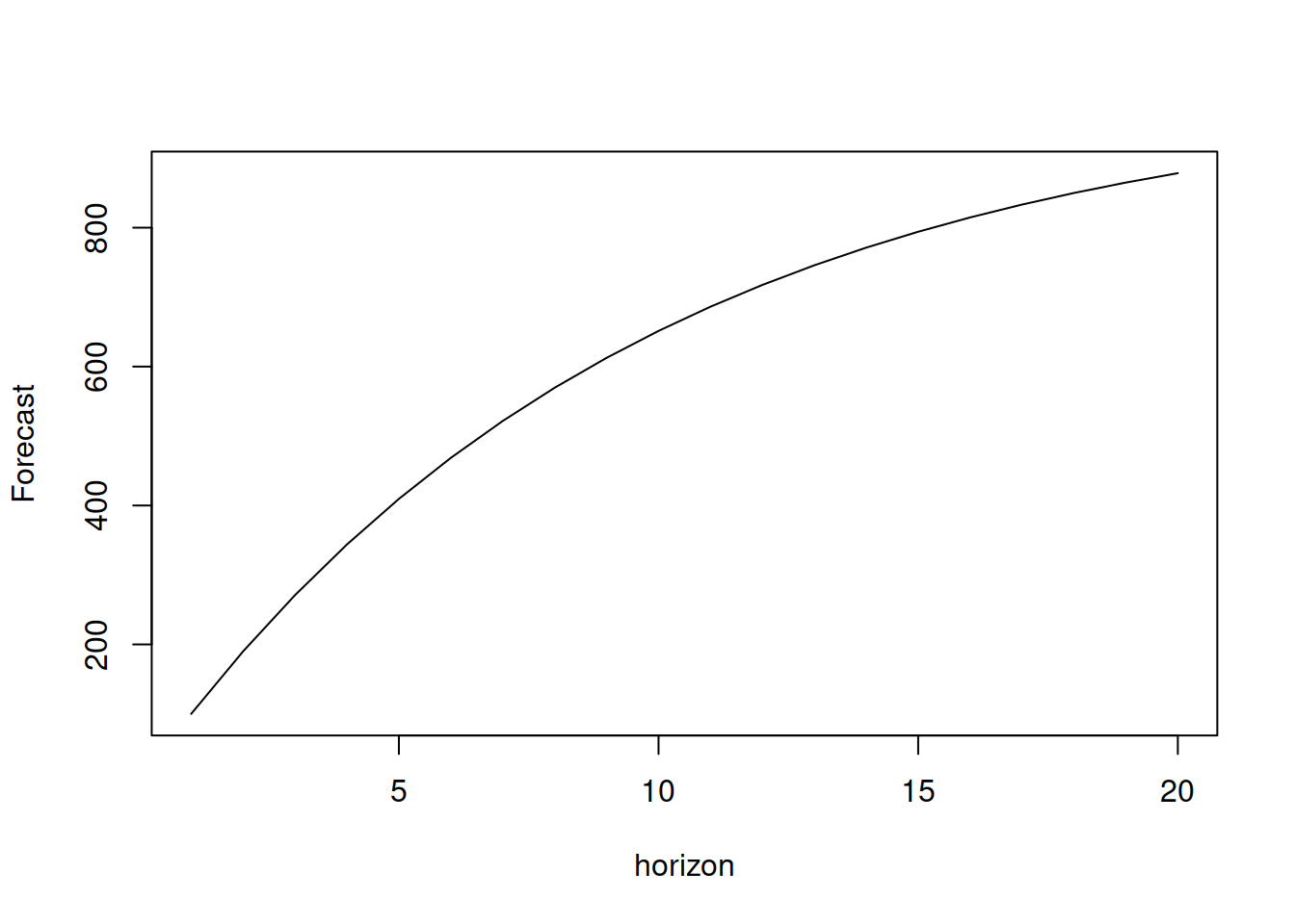
Figure 8.6: Forecast trajectory for an ARMA(1,1) model with constant.
The more complicated ARMA(p,q) models with p>1 will have more complex trajectories with potential harmonics, but the idea of dampening in the AR(p) part of the model stays.
An example of time series generated from ARMA(3,3) with constant is provided in Figure 8.7.
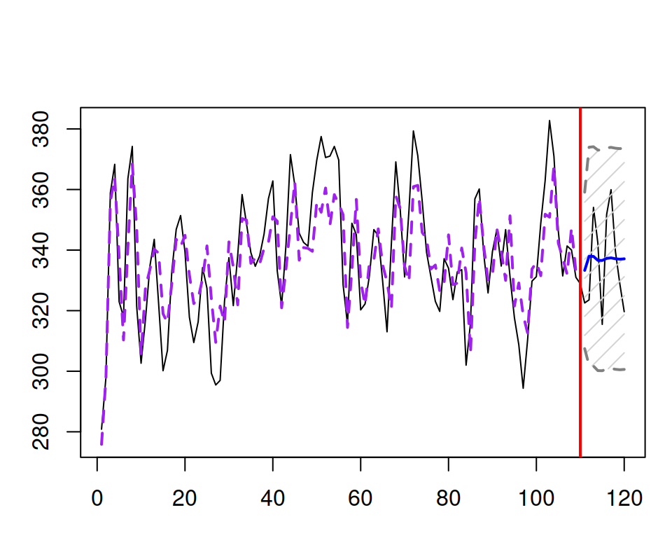
Figure 8.7: An example of an ARMA(3,3) with constant series and a forecast for it.
Finally, as alternative to adding \(a_0\), each actual value of \(y_t\) can be centred via \(y^\prime_t = y_t -\bar{y}\), where \(\bar{y}\) is the in-sample mean, making sure that the mean of \(y^\prime_t\) is zero and ARMA can be applied to the \(y^\prime_t\) data instead of \(y_t\). However, this approach introduces additional steps, but the result on stationary data is typically the same as adding the constant.
8.1.5 I(d)
Based on the previous discussion, we can conclude that ARMA cannot be efficiently applied to non-stationary data. So, if we deal with one, we need to make it stationary. The conventional way of doing that is by taking differences in the data. The logic behind this is straightforward: if the data is not stationary, the mean somehow changes over time. This can be, for example, due to a trend in the data. In this case, we should be talking about the change of variable \(y_t\) rather than the variable itself. So we should work on the following data instead: \[\begin{equation} \Delta y_t = y_t -y_{t-1} = y_t (1 -B), \tag{8.20} \end{equation}\] if the first differences have a constant mean. The simplest model with differences is I(1), which is also known as the Random Walk (see Section 3.3.1): \[\begin{equation} \Delta y_t = \epsilon_t. \tag{8.21} \end{equation}\] It can also be reformulated in a simpler, more interpretable form by inserting (8.20) in (8.21) and regrouping elements: \[\begin{equation} y_t = y_{t-1} + \epsilon_t. \tag{8.22} \end{equation}\] The model (8.22) can also be perceived as AR(1) with \(\phi_1=1\). This is a non-stationary model (meaning that the unconditional mean of \(y_t\) is not constant) and the point forecast from it corresponds to the one from the Naïve method (see Section 3.3.1) with a straight line equal to the last observed actual value (again, assuming that \(\mathrm{E}(\epsilon_{t})=0\) and that the other basic assumptions from Section 1.4.1 hold): \[\begin{equation} \mathrm{E}(y_{t+h}|t) = \mathrm{E}(y_{t+h-1}|t) + \mathrm{E}(\epsilon_{t+h}|t) = y_{t} . \tag{8.23} \end{equation}\] Visually, the Random Walk data and the forecast from it are shown in Figure 8.8.
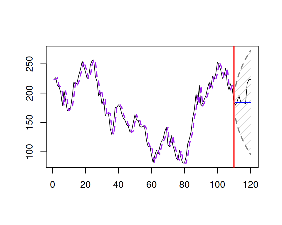
Figure 8.8: A Random Walk data example.
Another simple model that relies on differences of the data is called Random Walk with drift (which was discussed in Section 3.3.4) and is formulated by adding constant \(a_0\) to the right-hand side of equation (8.21): \[\begin{equation} \Delta y_t = a_0 + \epsilon_t. \tag{8.24} \end{equation}\] This model has some similarities with the global level model, which is formulated via the actual value rather than differences (see Section 3.3.2): \[\begin{equation*} {y}_{t} = a_0 + \epsilon_t. \end{equation*}\] Using a similar regrouping as with the Random Walk, we can obtain a simpler form of (8.24): \[\begin{equation} y_t = a_0 + y_{t-1} + \epsilon_t , \tag{8.25} \end{equation}\] which is, again, equivalent to the AR(1) model with \(\phi_1=1\), but this time with a constant. The term “drift” appears because \(a_0\) acts as an additional element, showing the tendency in the data: if it is positive, the model will exhibit a positive trend; if it is negative, the trend will be negative. This can be seen for the conditional mean, for example, for the case of \(h=2\): \[\begin{equation} \mathrm{E}(y_{t+2}|t) = \mathrm{E}(a_0) + \mathrm{E}(y_{t+1}|t) + \mathrm{E}(\epsilon_{t+2}|t) = a_0 + \mathrm{E}(a_0 + y_t + \epsilon_t|t) = 2 a_0 + y_t , \tag{8.26} \end{equation}\] or in general for the horizon \(h\): \[\begin{equation} \mathrm{E}(y_{t+h}|t) = h a_0 + y_t . \tag{8.27} \end{equation}\] Visually, the data and the forecast from it are shown in Figure 8.9.
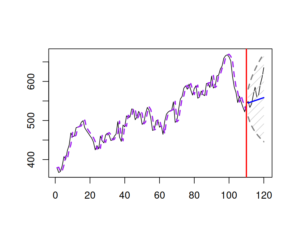
Figure 8.9: A Random Walk with drift with \(a_0=2\).
In a manner similar to (8.20), we can also introduce second differences of the data (differences of differences) if we suspect that the change of variable over time is not stationary, which would be written as: \[\begin{equation} \Delta^2 y_t = \Delta y_t -\Delta y_{t-1} = y_t -y_{t-1} -y_{t-1} + y_{t-2}, \tag{8.28} \end{equation}\] or using the backshift operator: \[\begin{equation} \Delta^2 y_t = y_t(1 -2B + B^2) = y_t (1 -B)^2. \tag{8.29} \end{equation}\] In fact, we can introduce higher level differences if we want to (but typically we should not) based on the idea of (8.29): \[\begin{equation} \Delta^d = (1-B)^d. \tag{8.30} \end{equation}\] Using (8.30), the I(d) model is formulated as: \[\begin{equation} \Delta^d y_t = \epsilon_t. \tag{8.31} \end{equation}\]
8.1.6 ARIMA(p,d,q)
Finally, having made the data stationary via the differences, we can introduce ARMA elements (8.14) to it which would be done on the differenced data, instead of the original \(y_t\): \[\begin{equation} y_t \Delta^d(B) \varphi^p(B) = \epsilon_t \vartheta^q(B) , \tag{8.32} \end{equation}\] or in a more general form (8.12) with (8.30): \[\begin{equation} y_t (1-B)^d (1 -\phi_1 B -\dots -\phi_p B^p) = \epsilon_t (1 + \theta_1 B + \dots + \theta_q B^q), \tag{8.33} \end{equation}\] which is an ARIMA(p,d,q) model. This model allows producing trends with some values of differences and also inherits the trajectories from both AR(p) and MA(q). This implies that the point forecasts from the model can exhibit complicated trajectories, depending on the values of p, d, q, and the model’s parameters.
The model (8.33) is difficult to interpret in a general form, but opening the brackets and moving all elements but \(y_t\) to the right-hand side helps understanding each specific model.
Figure 8.10 demonstrates how data would look if it was generated from ARIMA(1,1,2) and how the forecasts would look if the same model ARIMA(1,1,2) was applied to the data. Because of the AR(1) term in the model, its forecast trajectory is dampening, similar to how it was done in the ETS(A,Ad,N) model.
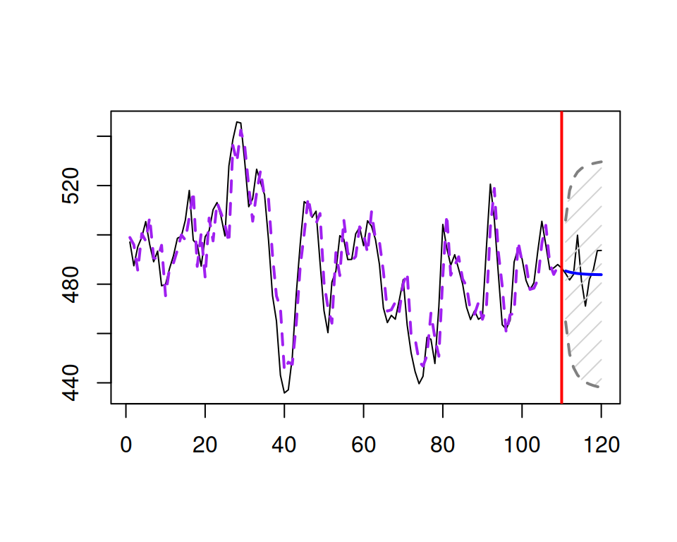
Figure 8.10: An example of ARIMA(1,1,2) data and a forecast for it.
8.1.7 Parameters’ bounds
ARMA models have two conditions that need to be satisfied for them to be useful and to work appropriately:
- Stationarity;
- Invertibility.
Condition (1) has already been discussed in Section 8.1. It is imposed on the model’s AR parameters, ensuring that the forecast trajectories do not exhibit explosive behaviour (in terms of both mean and variance). (2) is equivalent to the stability condition in ETS (Section 5.4) and refers to the MA parameters: it guarantees that the old observations do not have an increasing impact on the recent ones. The term “invertibility” comes from the idea that any MA process can be represented as an infinite AR process via the inversion of the parameters as long as the parameters lie in some specific bounds. For example, an MA(1) model, which is written as: \[\begin{equation} y_t = \epsilon_t + \theta_1 \epsilon_{t-1} = \epsilon_t (1 + \theta_1 B) , \tag{8.34} \end{equation}\] can be rewritten as: \[\begin{equation} y_t (1 + \theta_1 B)^{-1} = \epsilon_t, \tag{8.35} \end{equation}\] or in a slightly easier to digest form (based on (8.34) and the idea that \(\epsilon_{t} = y_{t} -\theta_1 \epsilon_{t-1}\), implying that \(\epsilon_{t-1} = y_{t-1} -\theta_1 \epsilon_{t-2}\)): \[\begin{equation} y_t = \theta_1 y_{t-1} -\theta_1^2 \epsilon_{t-2} + \epsilon_t = \theta_1 y_{t-1} -\theta_1^2 y_{t-2} + \theta_1^3 \epsilon_{t-2} + \epsilon_t = \sum_{j=1}^\infty -1^{j-1} \theta_1^j y_{t-j} + \epsilon_t. \tag{8.36} \end{equation}\] The recursion in (8.36) shows that the recent actual value \(y_t\) depends on the previous infinite number of values of \(y_{t-j}\) for \(j=\{1,\dots,\infty\}\). The parameter \(\theta_1\), in this case, is exponentiated to the power \(j\) and leads to the exponential distribution of weights in this infinite series (looks similar to SES from Section 3.4, doesn’t it?). The invertibility condition makes sure that those weights decline over time with the increase of \(j\) so that the older observations do not have an increasing impact on the most recent \(y_t\).
There are different ways to check both conditions, the conventional one is by calculating the roots of the polynomial equations: \[\begin{equation} \begin{aligned} & \varphi^p(B) = 0 \text{ for AR} \\ & \vartheta^q(B) = 0 \text{ for MA} \end{aligned} , \tag{8.37} \end{equation}\] or expanding the functions in (8.37) and substituting \(B\) with a variable \(x\) (for convenience): \[\begin{equation} \begin{aligned} & 1 -\phi_1 x -\phi_2 x^2 -\dots -\phi_p x^p = 0 \text{ for AR} \\ & 1 + \theta_1 x + \theta_2 x^2 + \dots + \theta_q x^q = 0 \text{ for MA} \end{aligned} . \tag{8.38} \end{equation}\] Solving the first equation for \(x\) in (8.38), we get \(p\) roots (some of them might be complex numbers). For the model to be stationary, all the roots must be greater than one by absolute value. Similarly, if all the roots of the second equation in (8.38) are greater than one by absolute value, then the model is invertible (aka stable).
Calculating roots of polynomials is a difficult task, so there are simpler special cases for both conditions that guarantee that the more complicated ones are satisfied: \[\begin{equation} \begin{aligned} & 0 < \sum_{j=1}^p \phi_j < 1 \\ & 0 < \sum_{j=1}^q \theta_j < 1 \end{aligned} . \tag{8.39} \end{equation}\] But note that the condition (8.39) is rather restrictive and is not generally applicable for all ARIMA models. It can be used to skip the check of the more complicated condition (8.38) if it is satisfied by a set of estimated parameters.
Finally, in a special case with an AR(p) model with \(0 < \phi_j < 1\) for all \(j\) and \(\sum_{j=1}^p \phi_j = 1\), we end up with the moving weighted average, which is a non-stationary model. This becomes apparent from the connection between Simple Moving Average and AR processes (Svetunkov and Petropoulos, 2018).