13.3 The complete ADAM
Uniting demand occurrence (from Section 13.1) with the demand sizes (Section 13.2) parts of the model, we can now discuss the complete ADAM model, which in the most general form can be represented as: \[\begin{equation} \begin{aligned} & y_t = o_t z_t , \\ & {z}_{t} = w_z(\mathbf{v}_{z,t-\boldsymbol{l}}) + r_z(\mathbf{v}_{z,t-\boldsymbol{l}}) \epsilon_{z,t} \\ & \mathbf{v}_{z,t} = f_z(\mathbf{v}_{z,t-\boldsymbol{l}}) + g_z(\mathbf{v}_{z,t-\boldsymbol{l}}) \epsilon_{z,t} \\ & \\ & o_t \sim \text{Bernoulli} \left(p_t \right) , \\ & p_t = f_p(\mu_{a,t}, \mu_{b,t}) \\ & a_t = w_a(\mathbf{v}_{a,t-\boldsymbol{l}}) + r_a(\mathbf{v}_{a,t-\boldsymbol{l}}) \epsilon_{a,t} \\ & \mathbf{v}_{a,t} = f_a(\mathbf{v}_{a,t-\boldsymbol{l}}) + g_a(\mathbf{v}_{a,t-\boldsymbol{l}}) \epsilon_{a,t} \\ & b_t = w_b(\mathbf{v}_{b,t-\boldsymbol{l}}) + r_b(\mathbf{v}_{b,t-\boldsymbol{l}}) \epsilon_{b,t} \\ & \mathbf{v}_{b,t} = f_b(\mathbf{v}_{b,t-\boldsymbol{l}}) + g_b(\mathbf{v}_{b,t-\boldsymbol{l}}) \epsilon_{b,t} \end{aligned} , \tag{13.26} \end{equation}\] where the elements of the demand size and demand occurrence parts have been discussed in Sections 13.2 and 13.1, respectively. The model (13.26) can also be considered a more general one than the conventional ADAM ETS and ARIMA models: if the probability of occurrence \(p_t\) is equal to one for all observations, then the model reverts to them.
Summarising the discussions in previous sections of this chapter, the complete ADAM has the following assumptions:
- The demand sizes variable \(z_t\) is continuous. This is a reasonable assumption for many contexts, including, for example, energy forecasting. But even when we deal with integer values, Svetunkov and Boylan (2023a) showed that such a model does not perform worse than count data models. And if the integer values are needed, Svetunkov and Boylan (2023a) demonstrated that rounding up quantiles from such a model is a reasonable and efficient approach that performs well in terms of forecasting accuracy and inventory performance;
- Potential demand size may change over time even when \(o_t=0\). This means that the states evolve even when demand is not observed;
- Demand sizes and demand occurrence are independent. This simplifies many derivations and makes the model estimable. If the assumption is violated, a different model with different properties would need to be constructed. My understanding of the problem tells me that the model (13.26) will work well even if this is violated, but I have not done any experiments in this direction.
Depending on the specific model for each part and restrictions on \(\mu_{a,t}\) and \(\mu_{b,t}\), we might have different types of iETS models. To distinguish one model from another, we introduce the notation of iETS models of the form “iETS(demand sizes model)\(_\text{type of occurrence}\)(model A type)(model B type)”. For example, in the iETS(M,N,N)\(_G\)(A,N,N)(M,M,N), the first brackets say that ETS(M,N,N) was applied to the demand sizes, and the underscored letter points out that this is the “general probability” model (Subsection 13.1.4), which has ETS(A,N,N) for the model A and ETS(M,M,N) for the model B. If only one demand occurrence part is used (either \(a_t\) or \(b_t\)), then the redundant brackets are dropped, and the notation is simplified. For example, iETS(M,N,N)\(_O\)(M,M,N) has only one part for demand occurrence, which is captured using the ETS(M,M,N) model. If the same type of model is used for both demand sizes and demand occurrence, then the second brackets can be dropped as well, simplifying this further to iETS(M,N,N)\(_O\) (odds ratio model with ETS(M,N,N) for both parts, Section 13.1.2). All these models are implemented in the adam() function for the smooth package in R.
Similar notations and principles can be used for models based on ARIMA. Note that oARIMA is not yet implemented in smooth, but in theory, a model like iARIMA(0,1,1)\(_O\)(1,1,2) could be constructed in the ADAM framework.
Furthermore, in some cases, we might have explanatory variables, such as promotions, prices, weather, etc. They would impact both demand occurrence and demand sizes. In ADAM, they are implemented in respective oes() and adam() functions. Remember that when you include explanatory variables in the occurrence part, you are modelling the probability of occurrence, not the occurrence itself. So, for example, a promotional effect in this situation would mean a higher chance of having sales. In some other situations, we might not need dynamic models, such as ETS and ARIMA, and can focus on static regression. While adam() supports this, the alm() function from the greybox might be more suitable in this situation. It supports similar parameters, but its occurrence parameter accepts either the type of transform (plogis for the logit model and pnorm for the probit one) or a previously estimated occurrence model (either from alm() or from oes()).
In addition, there might be some cases, when the demand itself happens at random, but the demand sizes are at the same time not random. This means that when someone buys a product, they buy a fixed amount of \(z\). Typically, in these situations \(z=1\), but there might be some cases with other values. An example of such a demand process is shown in Figure 13.8.
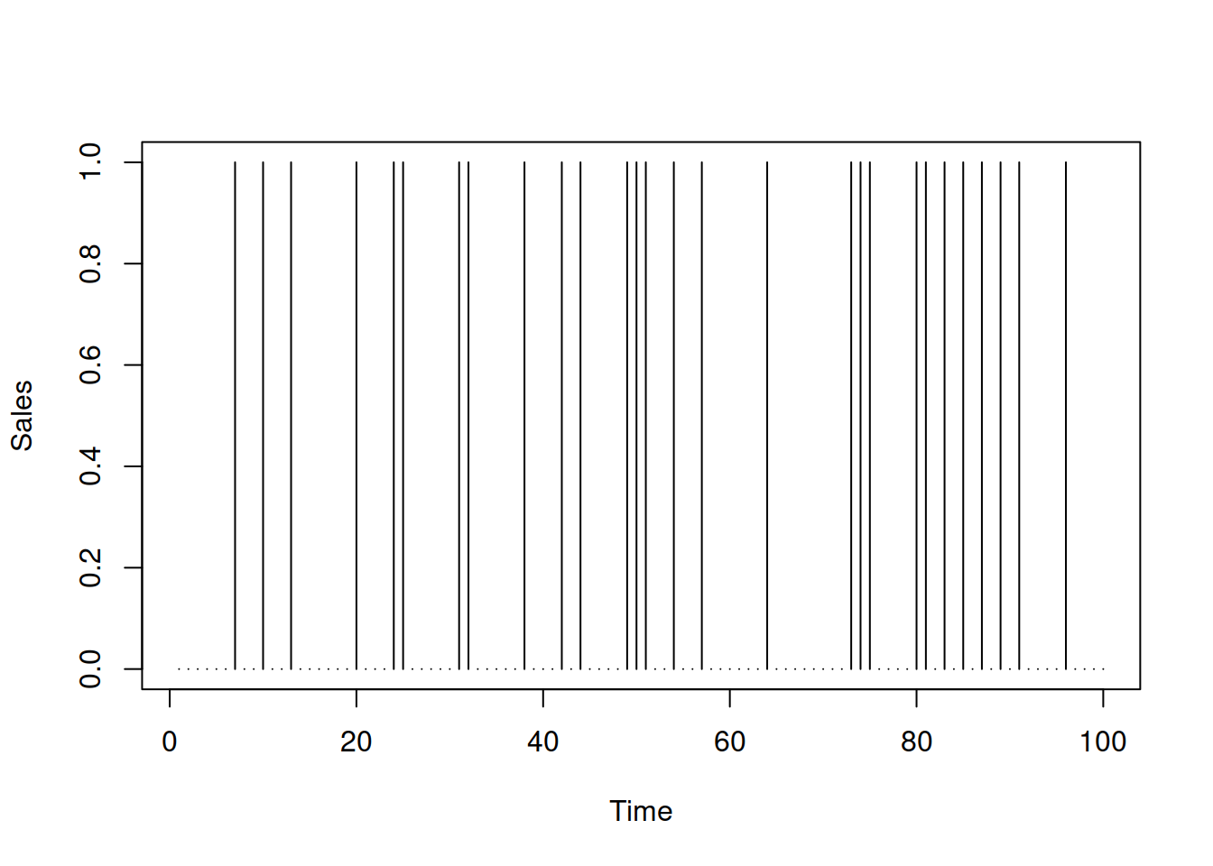
Figure 13.8: Example of intermittent time series with fixed demand sizes.
In this case, the model (13.26) simplifies to: \[\begin{equation} \begin{aligned} & y_t = o_t z , \\ & o_t \sim \text{Bernoulli} \left(p_t \right) \end{aligned} , \tag{13.27} \end{equation}\] where \(p_t\) can be captured via one of the demand occurrence models discussed in previous sections. Given that \(z\) is not random anymore, it does not require estimation, and the likelihood simplifies to the one for the demand occurrence (from Section 13.1). The forecast from this model can be generated by producing conditional expectation for the probability and then multiplying it by the value of \(z\).
Finally, in some situations the occurrence might be not random, i.e. we deal with not an intermittent demand, but with a demand, where sales sometimes do not happen (i.e. \(o_t=0\)), but we can predict perfectly when they happen. If we know when the demand occurs, we can use the respective values of zeroes and ones in the variable \(o_t\), simplifying the model (13.26) to:
\[\begin{equation}
\begin{aligned}
& y_t = o_t z_t , \\
& {z}_{t} = w_z(\mathbf{v}_{z,t-\boldsymbol{l}}) + r_z(\mathbf{v}_{z,t-\boldsymbol{l}}) \epsilon_{z,t} \\
& \mathbf{v}_{z,t} = f_z(\mathbf{v}_{z,t-\boldsymbol{l}}) + g_z(\mathbf{v}_{z,t-\boldsymbol{l}}) \epsilon_{z,t}
\end{aligned} ,
\tag{13.28}
\end{equation}\]
where the values of \(o_t\) are known in advance. An example of such a situation is the demand on watermelons, which reaches zero in specific periods of time in winter (at least in the UK). This special type of model is implemented in both the adam() and alm() functions, where the user needs to provide the vector of zeroes and ones in the occurrence parameter.
13.3.1 Maximum Likelihood Estimation
While there are different ways of estimating the parameters of the ADAM (13.26), it is worth focusing on likelihood estimation (Section 11.1) for consistency with other ADAMs. The likelihood of the model will consist of several parts:
- The probability density function (PDF) of demand sizes when demand occurs;
- The probability of occurrence;
- The probability of inoccurrence.
When demand occurs the likelihood is: \[\begin{equation} \mathcal{L}(\boldsymbol{\theta} | y_t, o_t=1) = p_t f_z(z_t | \mathbf{v}_{z,t-\boldsymbol{l}}) , \tag{13.29} \end{equation}\] while in the opposite case it is: \[\begin{equation} \mathcal{L}(\boldsymbol{\theta} | y_t, o_t=0) = (1-p_t) f_z(z_t | \mathbf{v}_{z,t-\boldsymbol{l}}), \tag{13.30} \end{equation}\] where \(\boldsymbol{\theta}\) includes all the estimated parameters of the model (for demand sizes and demand occurrence, including parameters of distribution, such as scale). Note that because the model assumes that the demand evolves over time even when it is not observed (\(o_t=0\)), we have a probability density function of demand sizes, \(f_z(z_t | \mathbf{v}_{z,t-\boldsymbol{l}})\) in (13.30). Based on equations (13.29) and (13.30), we can summarise the likelihood for the whole sample of \(T\) observations: \[\begin{equation} \mathcal{L}(\boldsymbol{\theta} | \textbf{y}) = \prod_{o_t=1} p_t \prod_{o_t=0} (1-p_t) \prod_{t=1}^T f_z(z_t | \mathbf{v}_{z,t-\boldsymbol{l}}) , \tag{13.31} \end{equation}\] or in logarithms: \[\begin{equation} \ell(\boldsymbol{\theta} | \textbf{y}) = \sum_{o_t=1} \log(p_t) + \sum_{o_t=0} \log(1-p_t) + \sum_{t=1}^T \log f_z(z_t | \mathbf{v}_{z,t-\boldsymbol{l}}), \tag{13.32} \end{equation}\] where \(\textbf{y}\) is the vector of all actual values and \(f_z(z_t | \mathbf{v}_{z,t-\boldsymbol{l}})\) can be substituted by a PDF of the assumed distribution from the list of candidates in Section 11.1. The main issue in calculating the likelihood (13.32) is that the demand sizes are not observable when \(o_t=0\). This means that we cannot calculate the likelihood using the conventional approach. We need to use something else. Svetunkov and Boylan (2023a) proposed using the Expectation Maximisation (EM) algorithm for this purpose, which is typically done in the following stages:
- Take Expectation of the likelihood;
- Maximise it with the obtained parameters;
- Go to (1) with the new set of parameters if the likelihood has not converged to the maximum.
A classic example with EM is when several samples have different parameters, and we need to split them (e.g. do clustering). In that case, we do not know what cluster specific observations belong to and what the probability that each observation belongs to one of the groups is. In our context, the problem is slightly different: we know probabilities, but we do not observe some of the values. As a result the application of EM gives a different result. If we take the expectation of (13.32) with respect to the unobserved demand sizes, we will get: \[\begin{equation} \begin{aligned} \mathrm{E}\left(\ell(\boldsymbol{\theta} | \textbf{y})\right) & = \sum_{o_t=1} \log f_z \left(z_{t} | \mathbf{v}_{z,t-\boldsymbol{l}} \right) + \sum_{o_t=0} \text{E} \left( \log f_z \left(z_{t} | \mathbf{v}_{z,t-\boldsymbol{l}} \right) \right) \\ & + \sum_{o_t=1} \log(p_t) + \sum_{o_t=0} \log(1- p_t) \end{aligned}. \tag{13.33} \end{equation}\] The first term in (13.33) is known because the \(z_t\) are observed when \(o_t=1\). The expectation in the second term of (13.33) is known in statistics as “Differential Entropy” (in the formula above, we have the negative differential entropy). It will differ from one distribution to another. Table 13.1 summarises differential entropies for the distributions used in ADAM.
| Assumption | Differential Entropy | |
|---|---|---|
| \(\epsilon_t \sim \mathcal{N}(0, \sigma^2)\) | \(\frac{1}{2}\left(\log(2\pi\sigma^2)+1\right)\) | |
| \(\epsilon_t \sim \mathcal{L}(0, s)\) | \(1+\log(2s)\) | |
| \(\epsilon_t \sim \mathcal{S}(0, s)\) | \(2+2\log(2s)\) | |
| \(\epsilon_t \sim \mathcal{GN}(0, s, \beta)\) | \(\beta^{-1}-\log\left(\frac{\beta}{2s\Gamma\left(\beta^{-1}\right)}\right)\) | |
| \(1+\epsilon_t \sim \mathcal{IG}(1, \sigma^2)\) | \(\frac{1}{2}\left(\log \left(\pi e \sigma^2\right) -\log(2) \right)\) | |
| \(1+\epsilon_t \sim \mathcal{\Gamma}(\sigma^{-2}, \sigma^2)\) | \(\sigma^{-2} + \log \Gamma\left(\sigma^{-2} \right) + \left(1-\sigma^{-2}\right)\psi\left(\sigma^{-2}\right)\) | |
| \(1+\epsilon_t \sim \mathrm{log}\mathcal{N}\left(-\frac{\sigma^2}{2}, \sigma^2\right)\) | \(\frac{1}{2}\left(\log(2\pi\sigma^2)+1\right)-\frac{\sigma^2}{2}\) |
The majority of formulae for differential entropy in Table 13.1 are taken from Lazo and Rathie (1978) with the exclusion of the one for \(\mathcal{IG}\), which was derived by Mudholkar and Tian (2002). These values can be inserted instead of the \(\text{E} \left( \log f_z \left(z_{t} | \mathbf{v}_{z,t-\boldsymbol{l}} \right) \right)\) in the formula (13.33), leading to the expected likelihood for respective distributions, which can then be maximised. For example, for Inverse Gaussian distribution (using the PDF from the Table 11.2 and the entropy from Table 13.1), we get: \[\begin{equation} \begin{aligned} \mathrm{E}\left(\ell(\boldsymbol{\theta} | \textbf{y})\right) & = -\frac{T_1}{2} \log \left(2 \pi \sigma^2 \right) -\frac{1}{2}\sum_{o_t=1} \left(1+\epsilon_{t}\right)^3 \\ & -\frac{3}{2} \sum_{o_t=1} \log y_t -\frac{1}{2 \sigma^2} \sum_{o_t=1} \frac{\epsilon_t^2}{1+\epsilon_t} \\ & -\frac{T_0}{2}\left(\log \pi e \sigma^2 -\log(2) \right) \\ & + \sum_{o_t=1} \log(p_t) + \sum_{o_t=0} \log(1- p_t) \end{aligned} , \tag{13.34} \end{equation}\] where \(T_0\) is the number of zeroes in the data and \(T_1\) is the number of non-zero values. Luckily, the EM process in our specific situation does not need to be iterative – the obtained likelihood can then be maximised directly by changing the values of parameters \(\boldsymbol{\theta}\). It is also possible to derive analytical formulae for parameters of some of distributions based on (13.33) and the values from Table 13.1. For example, in the case of the Inverse Gaussian distribution the estimate of scale parameter is: \[\begin{equation} \hat{\sigma}^2 = \frac{1}{T} \sum_{o_t=1}\frac{e_t^2}{1+e_t}. \tag{13.35} \end{equation}\] This is obtained by taking the derivative of (13.34) with respect to \(\sigma^2\) and equating it to zero. It can be shown that the likelihood estimates of scales for different distributions correspond to the conventional formulae from Section 11.1, but with the summation over \(o_t=1\) instead of all the observations. Note, however, that the division in (13.35) is done by the whole sample \(T\). This implies that the scale estimate will be biased, similarly to the classical bias of the sample variance. Svetunkov and Boylan (2023a) show that in the full ADAM, the estimate of scale is biased not only in-sample but also asymptotically, implying that with the increase of the sample size, it will be consistently lower than needed. This is because the summation is done over the non-zero values, while the division is done over the whole sample. This proportion of non-zeroes impacts the scale in (13.35), deflating its value. The only situation when the bias will be reduced is when the probability of occurrence reaches 1 (demand becomes regular). Still, the value (13.35) will maximise the expected likelihood (13.33) and is useful for inference. However, if one needs to construct prediction intervals, this bias needs to be addressed, which can be done using the conventional correction: \[\begin{equation} \hat{\sigma}^2{^{\prime}} = \frac{T}{T_1-k} \hat{\sigma}^2, \tag{13.36} \end{equation}\] where \(k\) is the number of all estimated parameters.
Finally, for the two exotic cases with known demand occurrence and known demand sizes, the likelihood (13.33) simplifies to the first two and the last two terms in the formula, respectively.
13.3.2 Conditional expectation and variance
Now that we have discussed how the model is formulated and how it can be estimated, we can move to the discussion of conditional expectation and variance from it. The former is needed to produce point forecasts, while the latter might be required for different inventory decisions.
The conditional \(h\) steps ahead expectation of the model can be obtained easily based on the assumption of independence of demand occurrence and demand sizes discussed earlier in Section 13.3: \[\begin{equation} \mathrm{E}(y_{t+h}|t) = \mu_{y,t+h|t} = \mathrm{E}(o_{t+h}|t) \mathrm{E}(z_{t+h}|t) = \mu_{o,t+h|t} \mu_{z,t+h|t}, \tag{13.37} \end{equation}\] where \(\mu_{o,t+h|t}\) is the conditional expectation of the occurrence variable (the conditional \(h\) steps ahead probability of occurrence) and \(\mu_{z,t+h|t}\) is the conditional expectation of the demand sizes variable \(z_t\). So, the forecast from the complete ADAM relies on the probability of occurrence of the variable and will reflect an average demand per period of time. As a result, it might be less than one in some cases, implying that the product is not sold every day. Consequentially, Kourentzes (2014) argued that the term “demand rate” should be used in this context instead of the conditional expectation. However, any forecasting model produces “demand per period” forecasts. They just typically assume that the probability of occurrence is equal to one (\(p_t=1\)) for all observations. So, there is no conceptual difference between the point forecasts produced by regular and intermittent demand models, and I do not see the point in using the “demand rate” term.
As for the conditional variance, it is slightly trickier than the conditional expectation, because the variance of a product involves not only variances, but expectations as well (assuming that two variables are independent): \[\begin{equation} \mathrm{V}(y_{t+h}|t) = \mathrm{V}(o_{t+h}|t) \mathrm{V}(z_{t+h|t}) + \mathrm{E}(o_{t+h}|t)^2 \mathrm{V}(z_{t+h}|t) + \mathrm{V}(o_{t+h}|t) \mathrm{E}(z_{t+h}|t)^2 . \tag{13.38}\end{equation}\] Given that we use Bernoulli distribution for the variable \(o_t\), its variance is equal to \(\mu_{o,t+h|t} (1-\mu_{o,t+h|t})\). In our context this implies that the conditional \(h\) steps ahead variance for the complete ADAM is: \[\begin{equation} \sigma^2_h = \mu_{o,t+h|t} (1-\mu_{o,t+h|t}) \sigma^2_{z,h} + \mu_{o,t+h|t}^2 \sigma^2_{z,h} + \mu_{o,t+h|t} (1-\mu_{o,t+h|t}) \mu_{z,t+h|t}^2 , \tag{13.39}\end{equation}\] or after some manipulations: \[\begin{equation} \sigma^2_h = \mu_{o,t+h|t} \left(\sigma^2_{z,h} + (1 -\mu_{o,t+h|t}) \mu_{z,t+h|t}^2 \right). \tag{13.40} \end{equation}\] All the elements of the formula (13.40) are available and have been discussed in Sections 5.3, 6.3, and 13.1.
When it comes to the two exotic cases, discussed in the beginning of this section, we have the following conditional expectation and variance:
When demand sizes are fixed and known, i.e. \(z_t=z\): \[\begin{equation} \begin{aligned} & \mu_{y,t+h|t} = \mu_{o,t+h|t} z, \\ & \sigma^2_h = \mu_{o,t+h|t} (1 -\mu_{o,t+h|t}) z^2 ; \end{aligned} \tag{13.41} \end{equation}\]
When demand occurrence is known: \[\begin{equation} \begin{aligned} & \mu_{y,t+h|t} = o_{t+h} \mu_{z,t+h|t}, \\ & \sigma^2_h = o_{t+h} \left(\sigma^2_{z,h} + (1 -o_{t+h}) \mu_{z,t+h|t}^2 \right). \end{aligned} \tag{13.42} \end{equation}\]
These two cases might not arise often, but it is important to understand how they change the moments of the model.