3.3 Simple forecasting methods
Now that we understand that time series might contain different components and that there are approaches for their decomposition, we can introduce several simple forecasting methods that can be used in practice, at least as benchmarks. Their usage aligns with the idea of forecasting principles discussed in Section 1.2. We discuss the most popular methods for the following specific types of time series:
- Level time series: Naïve (Subsection 3.3.1), Global Average (Subsection 3.3.2), Simple Moving Average (Subsection 3.3.3), Simple Exponential Smoothing (Section 3.4);
- Trend time series: Random Walk with drift (Subsection 3.3.4), Global Trend (Subsection 3.3.5);
- Seasonal time series: Seasonal Naïve (Subsection 3.3.6).
3.3.1 Naïve
Naïve is one of the simplest forecasting methods. According to it, the one-step-ahead forecast is equal to the most recent actual value: \[\begin{equation} \hat{y}_t = y_{t-1} . \tag{3.6} \end{equation}\] Using this approach might sound naïve indeed, but there are cases where it is very hard to outperform. Consider an example with temperature forecasting. If we want to know what the temperature outside will be in five minutes, then Naïve would be typically very accurate: the temperature in five minutes will be the same as it is right now.
The statistical model underlying Naïve is called the “Random Walk” and is written as: \[\begin{equation} y_t = y_{t-1} + \epsilon_t. \tag{3.7} \end{equation}\] The variability of \(\epsilon_t\) will impact the speed of change of the data: the higher it is, the more rapid the values will change. Random Walk and Naïve can be represented in Figure 3.8. In the example of R code below, we use the Simple Moving Average (discussed later in Subsection 3.3.3) of order 1 to generate the data from Random Walk and then produce forecasts using Naïve.
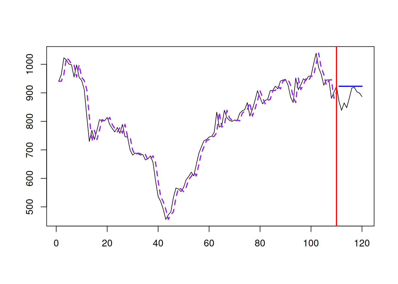
Figure 3.8: A Random Walk example.
As shown from the plot in Figure 3.8, Naïve lags behind the actual time series by one observation because of how it is constructed via equation (3.6). The point forecast corresponds to the straight line parallel to the x-axis. Given that the data was generated from Random Walk, the point forecast shown in Figure 3.8 is the best possible forecast for the time series, even though it exhibits rapid changes in the level.
Note that if the time series exhibits level shifts or other types of unexpected changes in dynamics, Naïve will update rapidly and reach the new level instantaneously. However, because it only has a memory of one (last) observation, it will not filter out the noise in the data but rather copy it into the future. So, it has limited usefulness in demand forecasting (although it has applications in financial analysis). However, being the simplest possible forecasting method, it is considered one of the basic forecasting benchmarks. If your model cannot beat it, it is not worth using.
3.3.2 Global Mean
While Naïve considers only one observation (the most recent one), the Global Mean (aka “global average”) relies on all the observations in the data: \[\begin{equation} \hat{y}_t = \bar{y} = \frac{1}{T} \sum_{t=1}^T y_{t} , \tag{3.8} \end{equation}\] where \(T\) is the sample size. The model underlying this forecasting method is called “global level” and is written as: \[\begin{equation} y_t = \mu + \epsilon_t, \tag{3.9} \end{equation}\] so that the \(\bar{y}\) is an estimate of the fixed expectation \(\mu\). Graphically, this is represented with a straight line going through the series as shown in Figure 3.9.
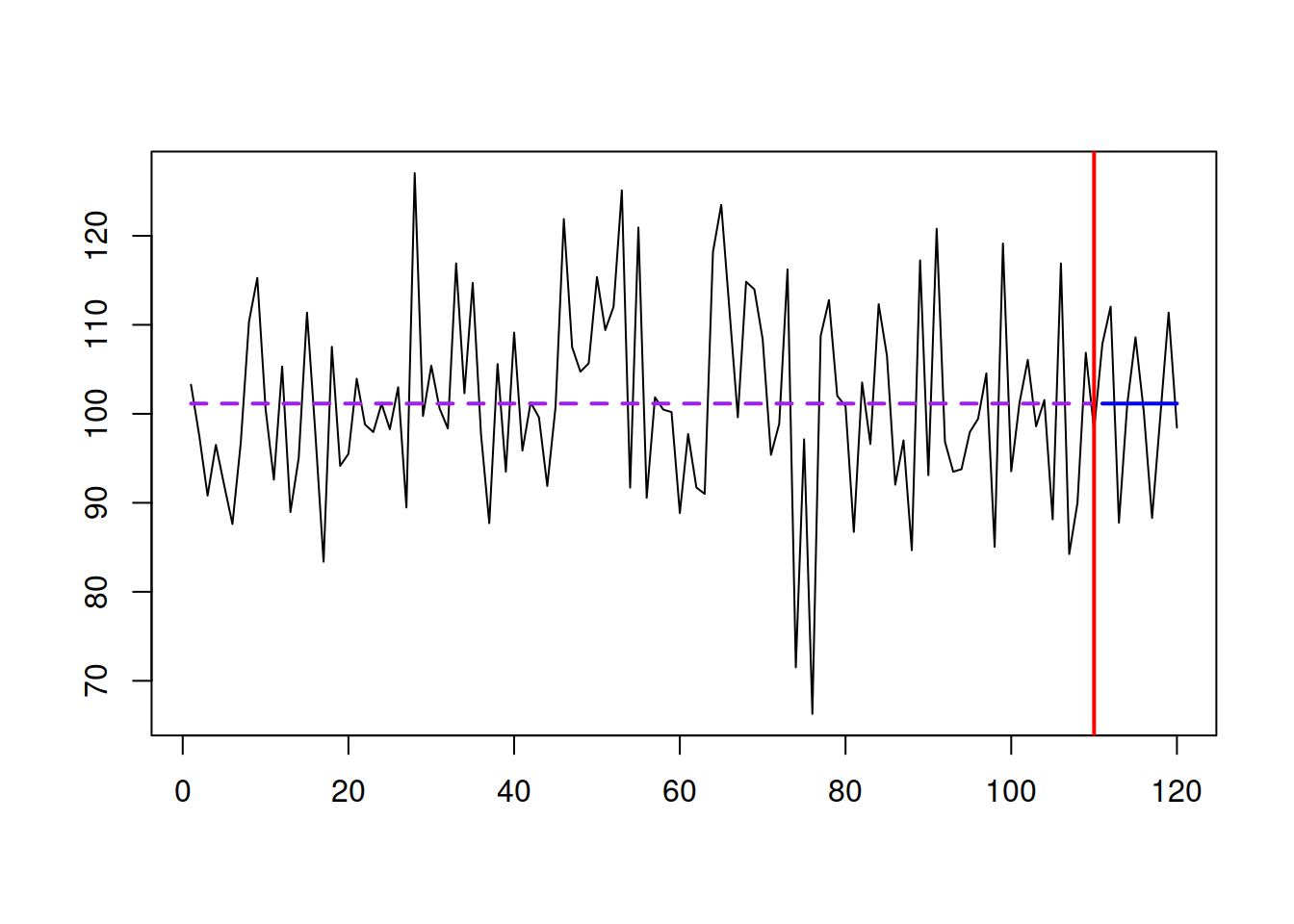
Figure 3.9: A global level example.
The series shown in Figure 3.9 is generated from the global level model, and the point forecast corresponds to the forecast from the Global Mean method. Note that the method assumes that the weights of the in-sample observations are equal, i.e. the first observation has precisely the exact weight of \(\frac{1}{T}\) as the last one (being as important as the last one). Suppose the series exhibits some changes in level over time. In that case, the Global Mean will not be suitable because it will produce the averaged out forecast, considering values for parts before and after the change. However, Global Mean works well in demand forecasting context and is a decent benchmark on intermittent data (discussed in Chapter 13).
3.3.3 Simple Moving Average
Naïve and Global Mean can be considered as opposite points in the spectrum of possible level time series (although there are series beyond Naïve, see for example ARIMA(0,1,1) with \(\theta_1>0\), discussed in Chapter 8). The series between them exhibits slow changes in level and can be modelled using different forecasting approaches. One of those is the Simple Moving Average (SMA), which uses the mechanism of the mean for a small part of the time series. It relies on the formula: \[\begin{equation} \hat{y}_t = \frac{1}{m}\sum_{j=1}^{m} y_{t-j}, \tag{3.10} \end{equation}\] which implies going through time series with something like a “window” of \(m\) observations and using their average for forecasting. The order \(m\) determines the length of the memory of the method: if it is equal to 1, then (3.10) turns into Naïve, while in the case of \(m=T\) it transforms into Global Mean. The order \(m\) is typically decided by a forecaster, keeping in mind that the lower \(m\) corresponds to the shorter memory method, while the higher one corresponds to the longer one.
Svetunkov and Petropoulos (2018) have shown that SMA has an underlying non-stationary AR(m) model with \(\phi_j=\frac{1}{m}\) for all \(j=1, \dots, m\). While the conventional approach to forecasting from SMA is to produce the straight line, equal to the last fitted value, Svetunkov and Petropoulos (2018) demonstrate that, in general, the point forecast of SMA does not correspond to the straight line. This is because to calculate several steps ahead point forecasts, the actual values in (3.10) are substituted iteratively by the predicted ones on the observations for the holdout.
y <- sim.sma(10,120)
par(mfcol=c(2,2), mar=c(2,2,2,1))
# SMA(1)
sma(y$data, order=1,
    h=10, holdout=TRUE) |>
    plot(which=7)
# SMA(10)
sma(y$data, order=10,
    h=10, holdout=TRUE) |>
    plot(which=7)
# SMA(20)
sma(y$data, order=20,
    h=10, holdout=TRUE) |>
    plot(which=7)
# SMA(110)
sma(y$data, order=110,
    h=10, holdout=TRUE) |>
    plot(which=7)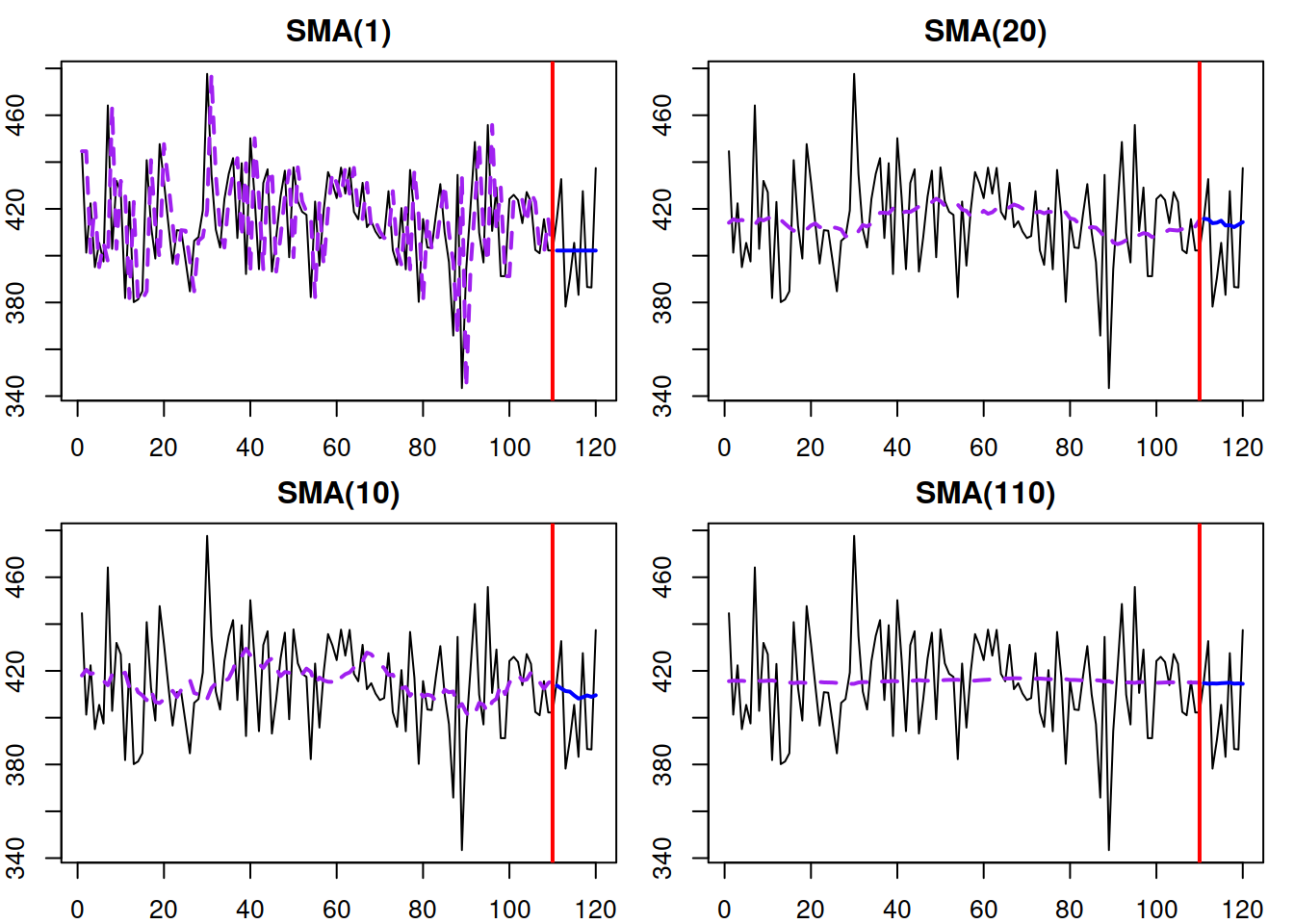
Figure 3.10: Examples of SMA time series and several SMA models of different orders applied to it.
Figure 3.10 demonstrates the time series generated from SMA(10) and several SMA models applied to it. We can see that the higher orders of SMA lead to smoother fitted lines and calmer point forecasts. On the other hand, the SMA of a very high order, such as SMA(110), does not follow the changes in time series efficiently, ignoring the potential changes in level. Given the difficulty with selecting the order \(m\), Svetunkov and Petropoulos (2018) proposed using information criteria for the order selection of SMA in practice.
Finally, an attentive reader has already spotted that the formula for SMA corresponds to the procedure of CMA of an odd order from equation (3.4). They are similar, but they have a different purpose: CMA is needed to smooth out the series, and the calculated values are inserted in the middle of the average, while SMA is used for forecasting, and the point forecasts are inserted at the last period of the average.
3.3.4 Random Walk with drift
So far, we have discussed the methods used for level time series. But as mentioned in Section 3.1, there are other components in the time series. In the case of the series with a trend, Naïve, Global Mean, and SMA will be inappropriate because they would be missing the essential component. The simplest model that can be used in this case is called “Random Walk with drift”, which is formulated as: \[\begin{equation} y_t = y_{t-1} + a_1 + \epsilon_t, \tag{3.11} \end{equation}\] where \(a_1\) is a constant term, the introduction of which leads to increasing or decreasing trajectories, depending on the value of \(a_1\). The point forecast from this model is calculated as: \[\begin{equation} \hat{y}_{t+h} = y_{t} + a_1 h, \tag{3.12} \end{equation}\] implying that the forecast from the model is a straight line with the slope parameter \(a_1\). Figure 3.11 shows what the data generated from Random Walk with drift and \(a_1=10\) looks like. This model is discussed in Subsection 8.1.5.
sim.ssarima(orders=list(i=1), lags=1, obs=120,
            constant=10) |>
    msarima(orders=list(i=1), constant=TRUE,
            h=10, holdout=TRUE) |>
    plot(which=7, main="")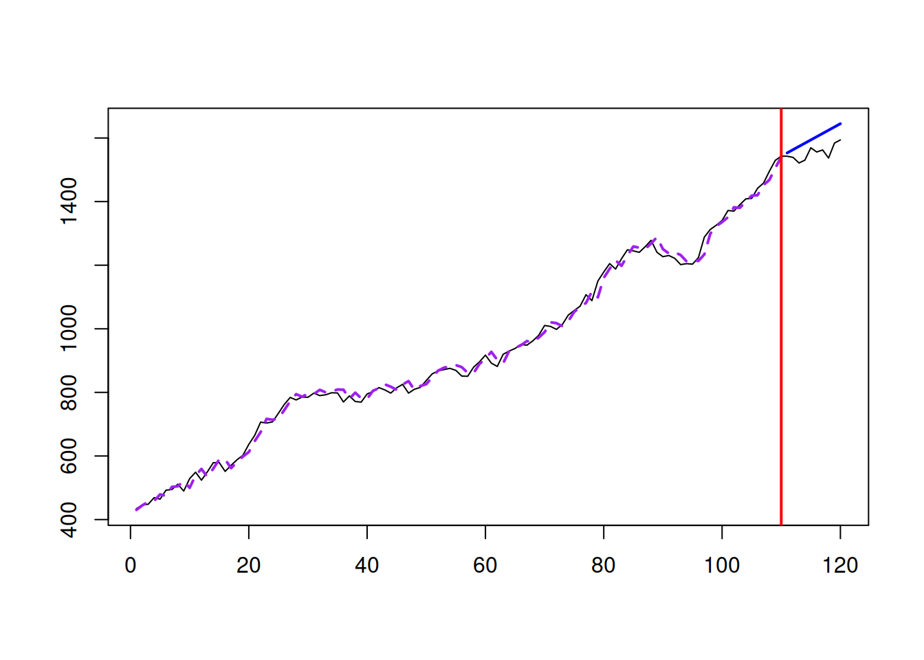
Figure 3.11: Random Walk with drift data and the model applied to that data.
The data in Figure 3.11 demonstrates a positive trend (because \(a_1>0\)) and randomness from one observation to another. The model is helpful as a benchmark and a special case for several other models because it is simple and requires the estimation of only one parameter.
3.3.5 Global Trend
Continuing the discussion of the trend time series, there is another simple model that is sometimes used in forecasting. The Global Trend model is formulated as: \[\begin{equation} y_t = a_0 + a_1 t + \epsilon_t, \tag{3.13} \end{equation}\] where \(a_0\) is the intercept and \(a_1\) is the slope of the trend. The positive value of \(a_1\) implies that the data exhibits growth, while the negative means decline. The size of \(a_1\) characterises the steepness of the slope. The point forecast from this model is: \[\begin{equation} \hat{y}_{t+h} = a_0 + a_1 (t+h), \tag{3.14} \end{equation}\] implying that the forecast from the model is a straight line with the slope parameter \(a_1\). Figure 3.12 shows how the data generated from a Global Trend with \(a_0=10\) and \(a_1=5\) looks like.
xreg <- data.frame(y=rnorm(120, 10+5*c(1:120), 10))
alm(y~trend, xreg, subset=c(1:100)) |>
    forecast(tail(xreg, 20), h=20) |>
    plot(main="")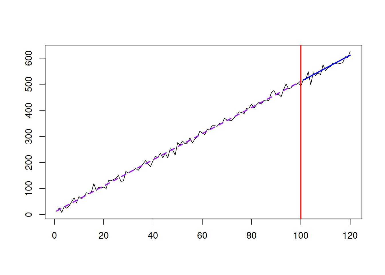
Figure 3.12: Global Trend data and the model applied to it.
The data in Figure 3.12 demonstrates a linear trend with some randomness around it. In this situation, the slope of the trend is fixed and does not change over time in contrast to what we observed in Figure 3.11 for a Random Walk with drift model. In some cases, the Global Trend model is the most suitable for the data. Some of the models discussed later in this monograph have the Global Trend as a special case when some restrictions on parameters are imposed (see, for example, Subsection 4.4.1).
3.3.6 Seasonal Naïve
Finally, in the case of seasonal data, there is a simple forecasting method that can be considered as a good benchmark in many situations. Similar to Naïve, Seasonal Naïve relies only on one observation, but instead of taking the most recent value, it uses the value from the same period a season ago. For example, for producing a forecast for January 1984, we would use January 1983. Mathematically this is written as: \[\begin{equation} \hat{y}_t = y_{t-m} , \tag{3.15} \end{equation}\] where \(m\) is the seasonal frequency. This method has an underlying model, Seasonal Random Walk: \[\begin{equation} y_t = y_{t-m} + \epsilon_t. \tag{3.16} \end{equation}\] Similar to Naïve, the higher variability of the error term \(\epsilon_t\) in (3.16) is, the faster the data exhibits changes. Seasonal Naïve does not require estimation of any parameters and thus is considered one of the popular benchmarks to use with seasonal data. Figure 3.13 demonstrates how the data generated from Seasonal Random Walk looks and how the point forecast from the Seasonal Naïve applied to this data performs.
y <- sim.ssarima(orders=list(i=1), lags=4,
                 obs=120, mean=0, sd=50)
msarima(y$data, orders=list(i=1), lags=4,
        h=10, holdout=TRUE) |>
    plot(which=7, main="")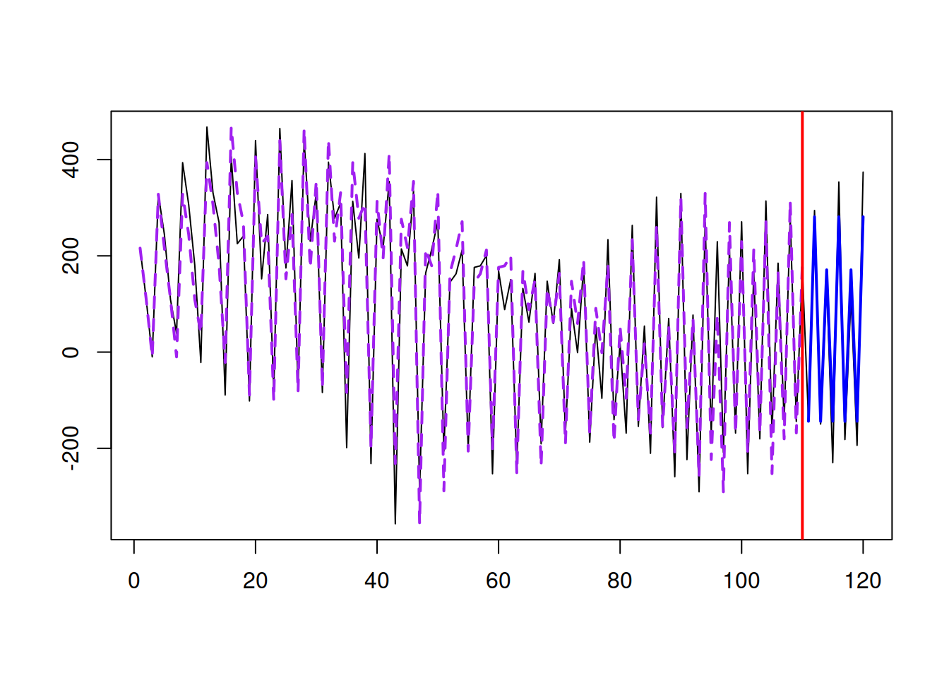
Figure 3.13: Seasonal Random Walk and Seasonal Naïve.
Similarly to the previous methods, if other approaches cannot outperform Seasonal Naïve, it is not worth spending time on those approaches.