14.7 Residuals are i.i.d.: Zero expectation
14.7.1 Unconditional expectation of residuals
This assumption only applies for the additive error models (Section 5.1). In the case of the multiplicative error models, it is changed to “expectation of the error term is equal to one” (Section 6.5). It does not make sense to check this assumption unconditionally because it does not mean anything in-sample: it will hold automatically for the residuals of a model in the case of OLS estimation. The observed mean of the residuals might not be equal to zero in other cases, but this does not give any helpful information. In fact, when we work with dynamic models (ETS, ARIMA), the in-sample residuals being equal to zero might imply for some of them that the final values of components are identical to the initial ones. For example, in the case of ETS(A,N,N) (from Section 4.3), we can use the transition equation from (4.3) to express the final value of level via the previous values up until \(t=0\): \[\begin{equation} \begin{aligned} \hat{l}_t = & \hat{l}_{t-1} + \hat{\alpha} e_t = \hat{l}_{t-2} + \hat{\alpha} e_{t-1} + \hat{\alpha} e_t = \\ & \hat{l}_0 + \hat{\alpha} \sum_{j=1}^t e_{t-j} . \end{aligned} \tag{14.3} \end{equation}\] If the mean of the residuals in-sample is indeed equal to zero, then the equation (14.3) reduces to \(\hat{l}_t=\hat{l}_0\). So, this assumption does not make sense in-sample and cannot be properly checked, meaning that it is all about the true model and the asymptotic behaviour rather than the model applied to data.
On the other hand, if for some reason the mean of residuals is not equal to zero in the population, then the model will change. For example, if we have an ETS(A,N,N) model with the non-zero mean of residuals \(\mu_\epsilon\), then the residuals can be represented in the form \(\epsilon_t = \mu_\epsilon + \xi_t\), where \(\mathrm{E}(\xi_t)=0\) which leads to a different model than ETS(A,N,N): \[\begin{equation} \begin{aligned} & y_t = l_{t-1} + \mu_\epsilon + \xi_t \\ & l_t = l_{t-1} + \alpha \mu_\epsilon + \alpha \xi_t \end{aligned}. \tag{14.4} \end{equation}\] If we apply an ETS(A,N,N) model to the data instead of (14.4), we will omit an important element and thus the estimated smoothing parameter will be higher than needed. The same logic applies to the multiplicative error models: the mean of residuals \(1+\epsilon_t\) should be equal to one for them, otherwise the model would change.
This phenomenon arises in dynamic models because of the “pull-to-centre” effect, where due to the presence of residuals in the transition equations, the model updates the states so that they become closer to the conditional mean of data.
Summarising this subsection, the expectation of residuals of ADAM should be equal to zero asymptotically, but it cannot be tested in-sample.
14.7.2 Conditional expectation of residuals
The more valuable part of this assumption that can be checked is whether the expectation of the residuals conditional on some variables (or time) equals to zero (or one in the case of a multiplicative error model). In a way, this comes to ensuring that there are no patterns in the residuals and thus there are no parts of data where residuals have systematically non-zero expectation.
There are different ways to diagnose this. First, we could use the already discussed plot of standardised (or studentised) residuals vs fitted values from Section 14.3. If the LOWESS line differs substantially from zero, we might suspect that the conditional expectation of residuals is not zero. Second, we could use the plot of residuals over time, which we have already discussed in Section 14.5. The logic here is similar to the previous one with the main difference being in spotting patterns, implying non-zero residuals over time. Furthermore, we can also plot residuals vs some of the variables to see if they cause the change in mean. But in a way, all of these methods might also mean that the residuals are autocorrelated and/or some transformations of variables are needed.
Related to the conditional expectation of the residuals, is the effect called “endogeneity” (discussed briefly in Section 15.3 of Svetunkov and Yusupova, 2025). According to the econometrics literature (see for example, Hanck et al., 2020), it implies that the residuals are correlated with some variables. This becomes equivalent to the situation when the expectation of residuals changes with the change of a variable. The most prominent cause of this effect is the omission of important variables (discussed in Section 14.1), which can sometimes be diagnosed by looking at correlations between the residuals and the omitted variables if the latter are available. While econometricians propose using other estimation methods (such as Instrumental Variables) to diminish the effect of endogeneity on regression models, the forecasters cannot do that because we need to fix the problem to get more reasonable forecasts rather than better estimates of parameters. Unfortunately, there is no universal recipe for the solution to this problem, but in some cases transforming variables, adding the omitted ones, or substituting them by proxies (variables that act similarly to the omitted ones) might resolve the issue to some extent.
14.7.3 Multistep forecast errors have zero mean
This follows from the previous assumption if the model is correctly specified and its residuals are i.i.d (also discussed in Subsection 14.5.1). In that situation, we would expect the multiple steps ahead forecast errors to have zero mean. In practice, this might be violated if some structural changes or level shifts are not taken into account by the model. The only thing to note is that the multistep forecast errors imply defining the forecast horizon \(h\). This should typically come from the task itself and the decisions made.
Practically speaking, the diagnostics of this assumption can be done using the rmultistep() method for adam(). This method would apply the estimated model and produce multiple steps ahead forecasts from each in-sample observation to the horizon \(h\), stacking the forecast errors in rows. Whether we use an additive or multiplicative error model, the method will produce the residual \(e_t\).
Here is an example of the code for the extraction and plotting of multistep forecast errors for the multiplicative model 5 from the previous sections:
# Extract multistep errors
adamSeat05ResidMulti <- rmultistep(adamSeat05, h=12)
# Give adequate names to the columns
colnames(adamSeat05ResidMulti) <- c(1:12)
# Produce boxplots
boxplot(adamSeat05ResidMulti, xlab="horizon")
# Add the zero line
abline(h=0, col="red")
# Add mean values
apply(adamSeat05ResidMulti,2,mean) |>
    points(col="red", pch=16)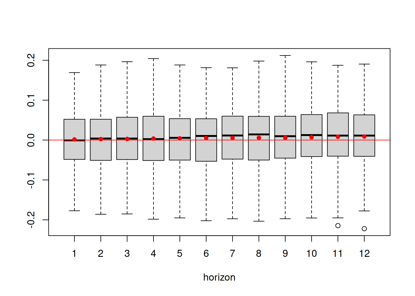
Figure 14.26: Boxplot of multistep forecast errors extracted from Model 5.
As the plot in Figure 14.26 demonstrates, the mean of the residuals does not increase substantially with the increase of the forecast horizon, which indicates that the model has captured the main structure in the data correctly.