11.2 Non MLE-based loss functions
An alternative approach for estimating ADAM is using the conventional loss functions, such as MSE, MAE, etc. In this case, the model selection using information criteria would not work, but this might not matter when you have already decided what model to use and want to improve it. Alternatively, you can use cross validation (e.g. rolling origin from Section 2.4) to select a model estimated using a non MLE-based loss function. But in some special cases, the minimisation of these losses would give the same results as the maximisation of some likelihood functions:
- MSE is minimised by mean, and its minimum corresponds to the maximum likelihood of Normal distribution (see discussion in Kolassa, 2016);
- MAE is minimised by median, and its minimum corresponds to the maximum likelihood of Laplace distribution (Schwertman et al., 1990);
- RMSLE is minimised by the geometric mean, and its minimum corresponds to the maximum likelihood of Log-Normal distribution (this is based on the fact that the maximum of the distribution coincides with the Normal one applied to the log-transformed data).
The main difference between using these losses and maximising respective likelihoods is in the number of estimated parameters: the latter implies that the scale is estimated together with the other parameters, while the former does not consider it and in a way provides it for free.
The assumed distribution does not necessarily depend on the used loss and vice versa. For example, we can assume that the actuals follow the Inverse Gaussian distribution, but estimate the model via minimisation of MAE. The estimates of parameters in this case might not be as efficient as in the case of MLE, but it is still possible to do.
When it comes to different types of models, the forecast error (which is used in respective losses) depends on the error type:
- Additive error: \(e_t = y_t -\hat{\mu}_{y,t}\);
- Multiplicative error: \(e_t = \frac{y_t -\hat{\mu}_{y,t}}{\hat{\mu}_{y,t}}\).
This follows directly from the respective ETS models.
11.2.1 MSE and MAE
MSE and MAE have been discussed in Section 2.1, but in the context of forecasts evaluation rather than estimation. If they are used for the latter, then the formulae (2.1) and (2.2) will be amended to: \[\begin{equation} \mathrm{MSE} = \sqrt{\frac{1}{T} \sum_{j=1}^T \left( e_t \right)^2 } \tag{11.7} \end{equation}\] and \[\begin{equation} \mathrm{MAE} = \frac{1}{T} \sum_{j=1}^T \left| e_t \right| , \tag{11.8} \end{equation}\] where the specific formula for \(e_t\) would depend on the error type as shown above. The main difference between the two estimators is in what they are minimised by: MSE is minimised by mean, while MAE is minimised by the median. This means that models estimated using MAE will typically be more conservative (i.e. in the case of ETS, have lower smoothing parameters). Gardner (2006) recommended using MAE in cases of outliers in the data, as the ETS model is supposed to become less reactive than in the case of MSE. Note that in case of intermittent demand, MAE should be in general avoided due to the issues discussed in Section 2.1.
11.2.2 HAM
Along with the discussed MSE and MAE, there is also HAM – “Half Absolute Moment” (Svetunkov et al., 2023b): \[\begin{equation} \mathrm{HAM} = \frac{1}{T} \sum_{j=1}^T \sqrt{\left|e_t\right|}, \tag{11.9} \end{equation}\] the minimum of which corresponds to the maximum likelihood of S distribution. The idea of this estimator is to minimise the errors that happen very often, close to the location of the distribution. It will typically ignore the outliers and focus on the most frequently appearing values. As a result, if used for the integer values, the minimum of HAM would correspond to the mode of that distribution if it is unimodal. I do not have a proof of this property, but it becomes apparent, given that the square root in (11.9) would reduce the influence of all values lying above one and increase the values of everything that lies between (0, 1) (e.g. \(\sqrt{0.16}=0.4\), but \(\sqrt{16}=4\)).
Similar to HAM, one can calculate other fractional losses, which would be even less sensitive to outliers and more focused on the frequently appearing values, e.g. by using the \(\sqrt[^\alpha]{\left|e_t\right|}\) with \(\alpha>1\). This would then correspond to the maximum of Generalised Normal distribution with shape parameter \(\beta=\frac{1}{\alpha}\).
11.2.3 LASSO and RIDGE
It is also possible to use LASSO (Tibshirani, 1996) and RIDGE for the estimation of ADAM (James et al., 2017 give a good overview of these losses with examples in R). This was studied in detail for ETS by Pritularga et al. (2023). The losses can be formulated in ADAM as: \[\begin{equation} \begin{aligned} \mathrm{LASSO} = &(1-\lambda) \sqrt{\frac{1}{T} \sum_{j=1}^T e_t^2} + \lambda \sum |\hat{\theta}| \\ \mathrm{RIDGE} = &(1-\lambda) \sqrt{\frac{1}{T} \sum_{j=1}^T e_t^2} + \lambda \sqrt{\sum \hat{\theta}^2}, \end{aligned} \tag{11.10} \end{equation}\] where \(\theta\) is the vector of all parameters in the model except for initial states of ETS and ARIMA components (thus, this includes all smoothing parameters, dampening parameter, AR, MA, and the initial parameters for the explanatory variables) and \(\lambda\) is the regularisation parameter. The idea of these losses is in the shrinkage of parameters. If \(\lambda=0\), then the losses become equivalent to the MSE, and when \(\lambda=1\), the optimiser would minimise the values of parameters, ignoring the MSE part. Pritularga et al. (2023) argues that the initial states of the model do not need to be shrunk (they will be handled by the optimiser automatically) and that the dampening parameter should shrink to one instead of zero (thus enforcing local trend model). Following the same idea, we introduce the following modifications of parameters in the loss in ADAM:
- The smoothing parameters should shrink towards zero, implying that the respective states will change slower over time (the model becomes less stochastic);
- Damping parameter is modified to shrink towards one, enforcing no dampening of the trend via \(\hat{\phi}^\prime=1-\hat{\phi}\);
- All AR parameters are forced to shrink to one: \(\hat{\phi}_i^\prime=1-\hat{\phi}_i\) for all \(i\). This means that ARIMA shrinks towards non-stationarity (this idea comes from the connection of ETS and ARIMA, discussed in Section 8.4);
- All MA parameters shrink towards zero, removing their impact on the model;
- If there are explanatory variables and the error term of the model is additive, then the respective parameters are divided by the standard deviations of the respective variables. In the case of the multiplicative error term, nothing is done because the parameters would typically be close to zero anyway (see a Chapter 10.1).
- Finally, in order to make \(\lambda\) slightly more meaningful, in the case of an additive error model, we also divide the MSE part of the loss by \(\mathrm{V}\left({\Delta}y_t\right)\), where \({\Delta}y_t=y_t-y_{t-1}\). This sort of scaling helps in cases when there is a trend in the data. We do not do anything for the multiplicative error models because, typically, the error is already small.
Remark. There is no good theory behind the shrinkage of AR and MA parameters. More research is required to understand how to shrink them properly.
Remark. The adam() function does not select the most appropriate lambda and will set it equal to zero if the user does not provide it. It is up to the user to try out different lambda and select the one that minimises a chosen error measure. This can be done, for example, using rolling origin procedure (Section 2.4).
11.2.4 Custom losses
It is also possible to use other non-standard loss functions for ADAM estimation. The adam() function allows doing that via the parameter loss. For example, we could estimate an ETS(A,A,N) model on the BJsales data using an absolute cubic loss (note that the parameters actual, fitted, and B are compulsory for the function):
lossFunction <- function(actual, fitted, B){
    return(mean(abs(actual-fitted)^3));
}
adam(BJsales, "AAN", loss=lossFunction, h=10, holdout=TRUE)
where actual is the vector of actual values \(y_t\), fitted is the estimate of the one-step-ahead point forecast \(\hat{y}_t\), and \(B\) is the vector of all estimated parameters, \(\hat{\theta}\). The syntax above allows using more advanced estimators, such as, for example, M-estimators (Barrow et al., 2020).
11.2.5 Examples in R
adam() has two parameters, one regulating the assumed distribution, and another one, regulating how the model will be estimated, and what loss will be used for these purposes. Here are examples with combinations of different losses and the Inverse Gaussian distribution for ETS(M,A,M) on AirPassengers data. We start with likelihood, MSE, MAE, and HAM:
adamETSMAMAir <- vector("list",6)
names(adamETSMAMAir) <-
    c("likelihood", "MSE", "MAE", "HAM", "LASSO", "Huber")
adamETSMAMAir[[1]] <- adam(AirPassengers, "MAM",h=12, holdout=TRUE,
                           distribution="dinvgauss",
                           loss="likelihood")
adamETSMAMAir[[2]] <- adam(AirPassengers, "MAM", h=12, holdout=TRUE,
                           distribution="dinvgauss",
                           loss="MSE")
adamETSMAMAir[[3]] <- adam(AirPassengers, "MAM", h=12, holdout=TRUE,
                           distribution="dinvgauss",
                           loss="MAE")
adamETSMAMAir[[4]] <- adam(AirPassengers, "MAM", h=12, holdout=TRUE,
                           distribution="dinvgauss",
                           loss="HAM")
In these cases, the models assuming the same distribution for the error term are estimated using likelihood, MSE, MAE, and HAM. Their smoothing parameters should differ, with MSE producing fitted values closer to the mean, MAE – closer to the median, and HAM – closer to the mode (but not exactly the mode) of the distribution.
In addition, we introduce ADAM ETS(M,A,M) estimated using LASSO with arbitrarily selected \(\lambda=0.9\):
adamETSMAMAir[[5]] <- adam(AirPassengers, "MAM", h=12, holdout=TRUE,
                           distribution="dinvgauss",
                           loss="LASSO", lambda=0.9)
And, finally, we estimate the same model using a custom loss, which in this case is Huber loss (Huber, 1992) with a threshold of 1.345:
# Huber loss with a threshold of 1.345
lossFunction <- function(actual, fitted, B){
    errors <- actual-fitted;
    return(sum(errors[errors<=1.345]^2) +
               sum(abs(errors)[errors>1.345]));
}
adamETSMAMAir[[6]] <- adam(AirPassengers, "MAM", h=12, holdout=TRUE,
                           distribution="dinvgauss",
                           loss=lossFunction)
Now we can compare the performance of the six models. First, we can compare the smoothing parameters:
##       likelihood   MSE   MAE   HAM LASSO Huber
## alpha      0.615 0.629 0.509 0.402     0 0.012
## beta       0.000 0.000 0.000 0.004     0 0.001
## gamma      0.283 0.255 0.448 0.058     0 0.087
What we observe in this case is that LASSO has the lowest smoothing parameter \(\alpha\) because it is shrunk directly in the model estimation. Also note that likelihood and MSE give similar values. They both rely on squared errors, but not in the same way because the likelihood of Inverse Gaussian distribution has some additional elements (see Section 11.1).
Unfortunately, we do not have information criteria for models 2 – 6 in this case because the likelihood function is not maximised with these losses, so it’s not possible to compare them via the in-sample statistics. But we can compare their holdout sample performance:
##     likelihood     MSE     MAE     HAM    LASSO   Huber
## ME      -6.077  -4.831 -10.357   1.636   44.730  16.126
## MAE     14.255  15.239  13.271  19.804   53.518  24.597
## MSE    426.253 448.958 376.721 745.216 3769.913 815.475
And we can also produce forecasts and plot them for the visual inspection (Figure 11.1):
adamETSMAMAirForecasts <- lapply(adamETSMAMAir, forecast,
                                 h=12, interval="empirical")
layout(matrix(c(1:6),3,2,byrow=TRUE))
for(i in 1:6){
    plot(adamETSMAMAirForecasts[[i]],
         main=paste0("ETS(MAM) estimated using ",
                     names(adamETSMAMAir)[i]))
}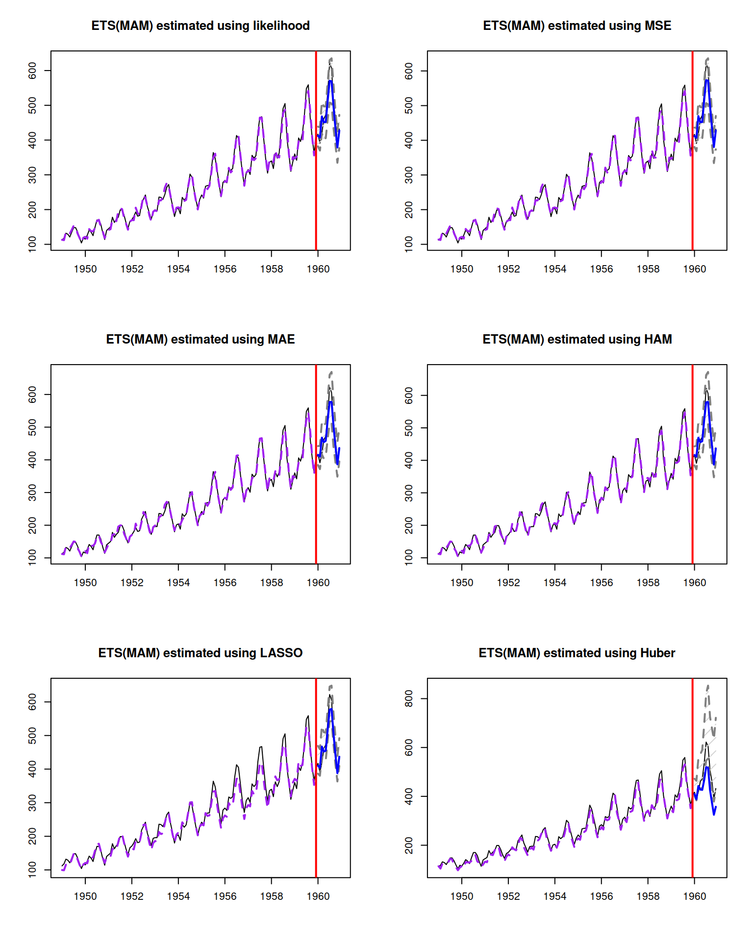
Figure 11.1: Forecasts from an ETS(M,A,M) model estimated using different loss functions.
What we observe in Figure 11.1 is that different losses led to different forecasts and prediction intervals (we used the empirical ones, discussed in Subsection 18.3.5). What can be done to make this practical is the rolling origin evaluation (Section 2.4) for different losses and then comparing forecast errors between them to select the most accurate approach.