5.6 Examples of application
5.6.1 Non-seasonal data
To see how the pure additive ADAM ETS works, we will try it out using the adam() function from the smooth package for R on Box-Jenkins sales data. We start with plotting the data:
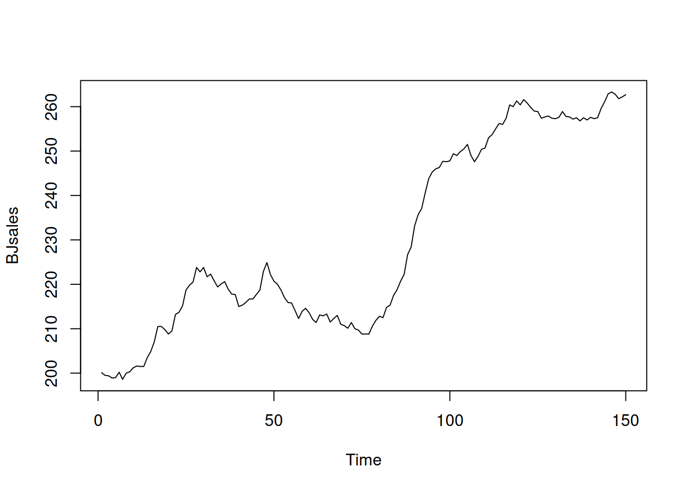
Figure 5.1: Box-Jenkins sales data.
The series in Figure 5.1 seem to exhibit a trend, so we will apply an ETS(A,A,N) model:
## Time elapsed: 0.01 seconds
## Model estimated using adam() function: ETS(AAN)
## With backcasting initialisation
## Distribution assumed in the model: Normal
## Loss function type: likelihood; Loss function value: 258.6072
## Persistence vector g:
##  alpha   beta
## 1.0000 0.2445
##
## Sample size: 150
## Number of estimated parameters: 3
## Number of degrees of freedom: 147
## Information criteria:
##      AIC     AICc      BIC     BICc
## 523.2144 523.3788 532.2463 532.6581
The model’s output summarises which specific model was constructed, what distribution was assumed, how the model was estimated, and also provides the values of smoothing parameters. It also reports the sample size, the number of parameters, degrees of freedom, and produces information criteria (see Section 16.4 of Svetunkov and Yusupova, 2025). We can compare this model with the ETS(A,N,N) to see which of them performs better in terms of information criteria (e.g. in terms of AICc):
## Time elapsed: 0.01 seconds
## Model estimated using adam() function: ETS(ANN)
## With backcasting initialisation
## Distribution assumed in the model: Normal
## Loss function type: likelihood; Loss function value: 273.0805
## Persistence vector g:
## alpha
##     1
##
## Sample size: 150
## Number of estimated parameters: 2
## Number of degrees of freedom: 148
## Information criteria:
##      AIC     AICc      BIC     BICc
## 550.1611 550.2427 556.1823 556.3868
In this situation the AICc for ETS(A,N,N) is higher than for ETS(A,A,N), so we should use the latter for forecasting purposes. We can produce point forecasts and a prediction interval (in this example we will construct 90% and 95% ones) and plot them (Figure 5.2):
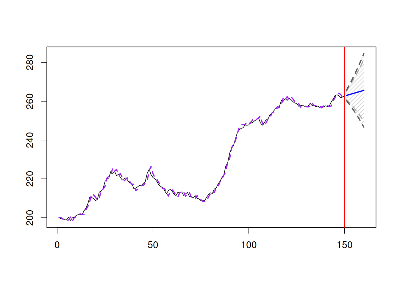
Figure 5.2: Forecast for Box-Jenkins sales data from ETS(A,A,N) model.
Notice that the bounds in Figure 5.2 are expanding fast, demonstrating that the components of the model exhibit high uncertainty, which is then reflected in the holdout sample. This is partially due to the high values of the smoothing parameters of ETS(A,A,N), with \(\alpha=1\). While we typically want to have lower smoothing parameters, in this specific case this might mean that the maximum likelihood is achieved in the admissible bounds (i.e. data exhibits even higher variability than we expected with the usual bounds). We can try it out and see what happens:
## Time elapsed: 0.02 seconds
## Model estimated using adam() function: ETS(AAN)
## With backcasting initialisation
## Distribution assumed in the model: Normal
## Loss function type: likelihood; Loss function value: 258.5197
## Persistence vector g:
##  alpha   beta
## 1.0378 0.2263
##
## Sample size: 150
## Number of estimated parameters: 3
## Number of degrees of freedom: 147
## Information criteria:
##      AIC     AICc      BIC     BICc
## 523.0394 523.2038 532.0713 532.4831
Both smoothing parameters are now higher, which implies that the uncertainty about the future values of states is higher as well, which is then reflected in the slightly wider prediction interval (Figure 5.3):

Figure 5.3: Forecast for Box-Jenkins sales data from an ETS(A,A,N) model with admissible bounds.
Although the values of smoothing parameters are higher than one, the model is still stable. In order to see that, we can calculate the discount matrix \(\mathbf{D}\) using the objects returned by the function to reflect the formula \(\mathbf{D}=\mathbf{F} -\mathbf{g}\mathbf{w}^\prime\):
(adamETSBJ$transition - adamETSBJ$persistence %*%
    adamETSBJ$measurement[nobs(adamETSBJ),,drop=FALSE]) |>
    eigen(only.values=TRUE)
## $values
## [1] 0.7841463 -0.0482092
##
## $vectors
## NULLNotice that the absolute values of both eigenvalues in the matrix are less than one, which means that the newer observations have higher weights than the older ones and that the absolute values of weights decrease over time, making the model stable.
If we want to test ADAM ETS with another distribution, it can be done using the respective parameter in the function (here we use Generalised Normal, estimating the shape together with the other parameters):
## Time elapsed: 0.03 seconds
## Model estimated using adam() function: ETS(AAN)
## With backcasting initialisation
## Distribution assumed in the model: Generalised Normal with shape=1.768
## Loss function type: likelihood; Loss function value: 258.369
## Persistence vector g:
## alpha  beta
## 1.000 0.245
##
## Sample size: 150
## Number of estimated parameters: 4
## Number of degrees of freedom: 146
## Information criteria:
##     AIC    AICc     BIC    BICc
## 524.739 525.014 536.781 537.472
Similar to the previous cases, we can plot the forecasts from the model:
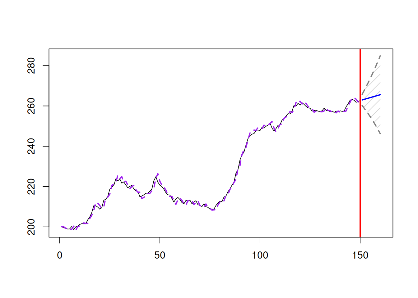
Figure 5.4: Forecast for Box-Jenkins sales data from an ETS(A,A,N) model with Generalised Normal distribution.
The prediction interval in this case is slightly wider than in the previous one, because the Generalised Normal distribution with \(\beta=\) 1.77 has fatter tails than the Normal one (Figure 5.4).
5.6.2 Seasonal data
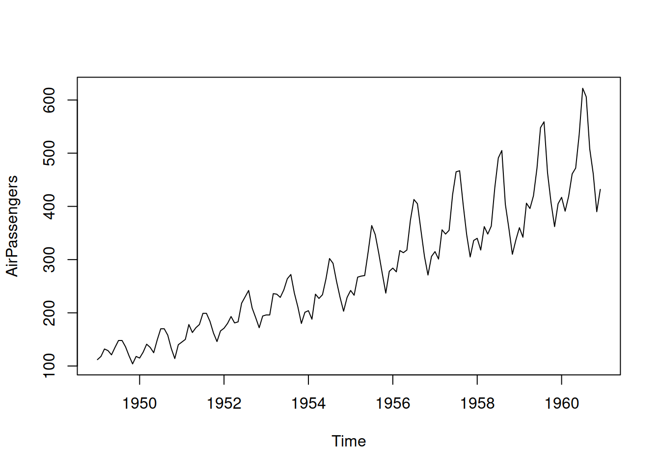
Figure 5.5: Air passengers data from Box-Jenkins textbook.
Now we will check what happens in the case of seasonal data. We use AirPassengers data, plotted in Figure 5.5, which apparently has multiplicative seasonality. But for demonstration purposes, we will see what happens when we use the wrong model with additive seasonality. We will withhold the last 12 observations to look closer at the performance of the ETS(A,A,A) model in this case:
Remark. In this specific case, the lags parameter is not necessary because the function will automatically get the frequency from the ts object AirPassengers. If we were to provide a vector of values instead of the ts object, we would need to specify the correct lag. Note that 1 (lag for level and trend) is unnecessary; the function will always use it anyway.
Remark. In some cases, the optimiser might converge to the local minimum, so if you find the results unsatisfactory, it might make sense to reestimate the model, tuning the parameters of the optimiser (see Section 11.4 for details). Here is an example (we increase the number of iterations in the optimisation and set new starting values for the smoothing parameters):
adamETSAir$B[1:3] <- c(0.2,0.1,0.3)
adamETSAir <- adam(AirPassengers, "AAA", lags=12,
                   h=12, holdout=TRUE,
                   B=adamETSAir$B, maxeval=1000)
adamETSAir
## Time elapsed: 0.03 seconds
## Model estimated using adam() function: ETS(AAA)
## With backcasting initialisation
## Distribution assumed in the model: Normal
## Loss function type: likelihood; Loss function value: 511.4407
## Persistence vector g:
## alpha beta gamma
## 0.252 0.000 0.748
##
## Sample size: 132
## Number of estimated parameters: 4
## Number of degrees of freedom: 128
## Information criteria:
## AIC AICc BIC BICc
## 1030.881 1031.196 1042.413 1043.182
##
## Forecast errors:
## ME: 5.861; MAE: 13.618; RMSE: 17.597
## sCE: 26.795%; Asymmetry: 53.9%; sMAE: 5.188%; sMSE: 0.449%
## MASE: 0.565; RMSSE: 0.562; rMAE: 0.179; rRMSE: 0.171Notice that because we fit the seasonal additive model to the data with multiplicative seasonality, the smoothing parameter \(\gamma\) has become large – the seasonal component needs to be updated frequently to keep up with the changing seasonal profile. In addition, because we use the holdout parameter, the function also reports the error measures for the point forecasts on that part of the data. This can be useful when comparing the performance of several models on a time series. And here is how the forecast from ETS(A,A,A) looks on this data:
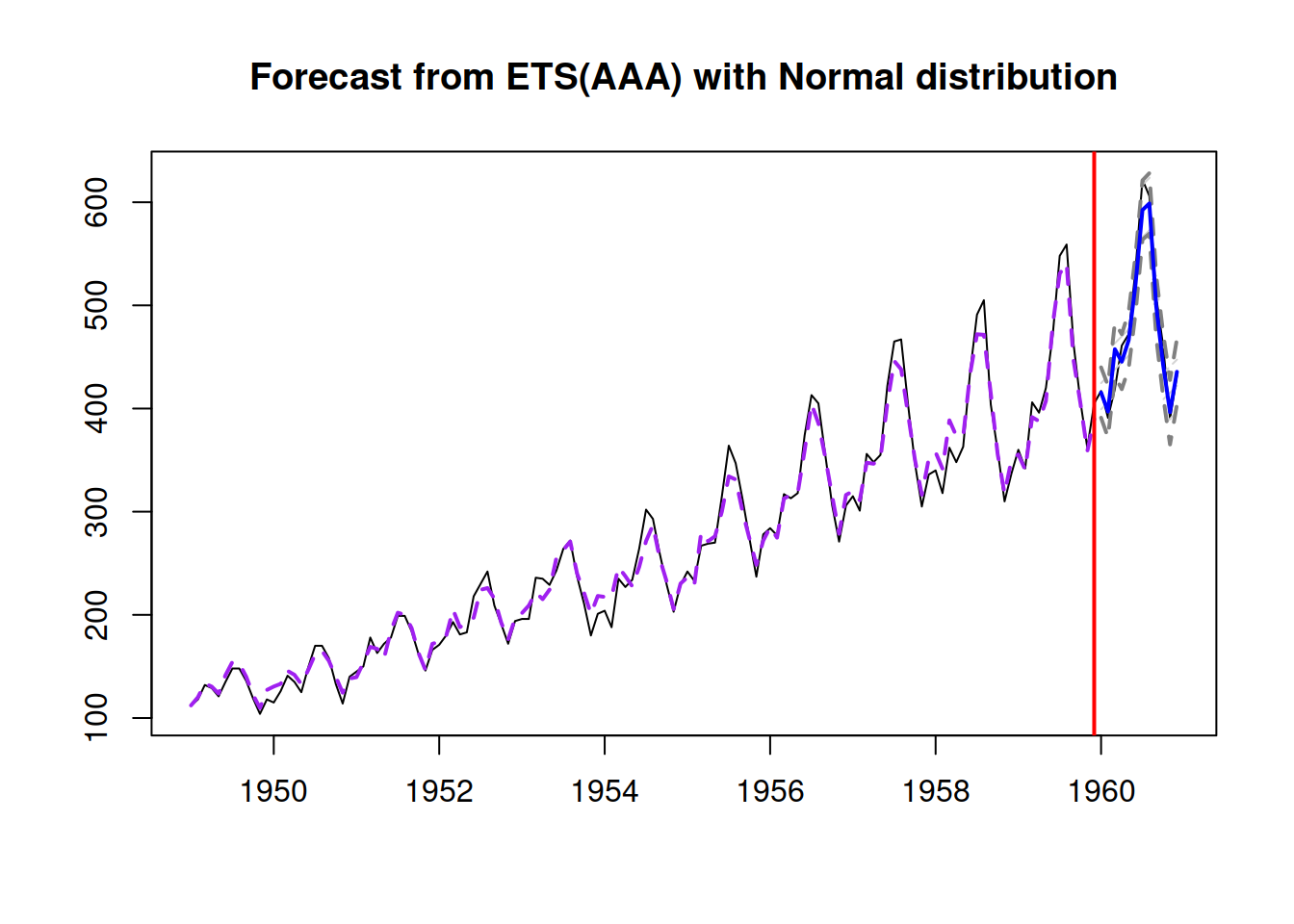
Figure 5.6: Forecast for air passengers data using an ETS(A,A,A) model.
Figure 5.6 demonstrates that while the fit to the data is far from perfect, due to a pure coincidence, the point forecast from this model is decent.
In order to see how the ADAM ETS decomposes the data into components, we can plot it via the plot() method with which=12 parameter:
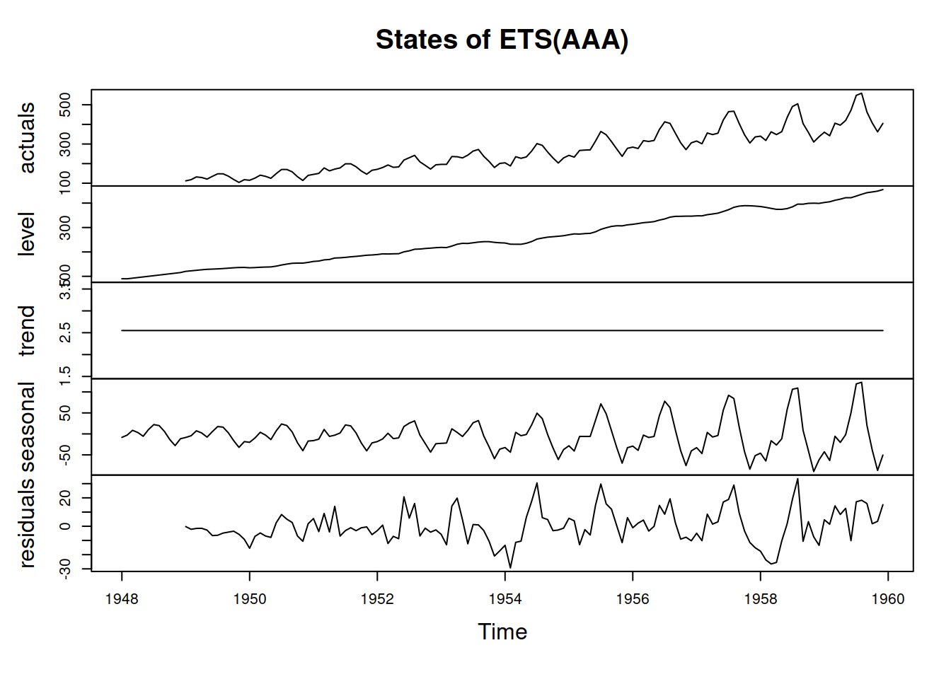
Figure 5.7: Decomposition of air passengers data using an ETS(A,A,A) model.
We can see on the graph in Figure 5.7 that the residuals still contain some seasonality, so there is room for improvement. This probably happened because the data exhibits multiplicative seasonality rather than the additive one. For now, we do not aim to fix this issue.