14.1 Model specification: Omitted variables
We start with one of the most critical assumptions for models: the model does not omit important variables. If it does then the point forecasts might not be as accurate as we would expect and in some serious cases exhibit substantial bias. For example, if the model omits a seasonal component, it will not be able to produce accurate forecasts for specific observations (e.g. months of year).
In general, this issue is difficult to diagnose because it is typically challenging to identify what is missing if we do not have it in front of us. The best thing one can do is a mental experiment, trying to comprise a list of all theoretically possible components and variables that would impact the variable of interest. If you manage to come up with such a list and realise that some of them are missing, the next step would be to collect the variables themselves or use their proxies. The proxies are variables that are expected to be correlated with the missing variables and can partially substitute them. We would need to add the missing information in the model one way or another.
In case of ETS components, the diagnostics of this issue is possible, because the pool of components is restricted and we know what the data with different components should look like (see Section 4.1). In the case of ARIMA, the diagnostics comes to analysing ACF/PACF (Section 14.5). But in the case of regression, it might be difficult to say what specifically is missing.
However, in some cases, we might be able to diagnose this even for the regression model. For example, with the model that we estimated in the previous section, we have a set of variables not included in it. A simple thing to do is to see if the residuals of our model are correlated with any of the omitted variables. We can either produce scatterplots or calculate measures of association (see Chapter 9 of Svetunkov and Yusupova, 2025) to see if there are relations in the residuals. I will use assoc() and spread() functions from greybox for this:
# Create a new matrix, removing the variables that are already
# in the model
SeatbeltsWithResiduals <-
  cbind(as.data.frame(residuals(adamSeat01)),
        Seatbelts[,-c(2,5,6)])
colnames(SeatbeltsWithResiduals)[1] <- "residuals"
# Spread plot
greybox::spread(SeatbeltsWithResiduals)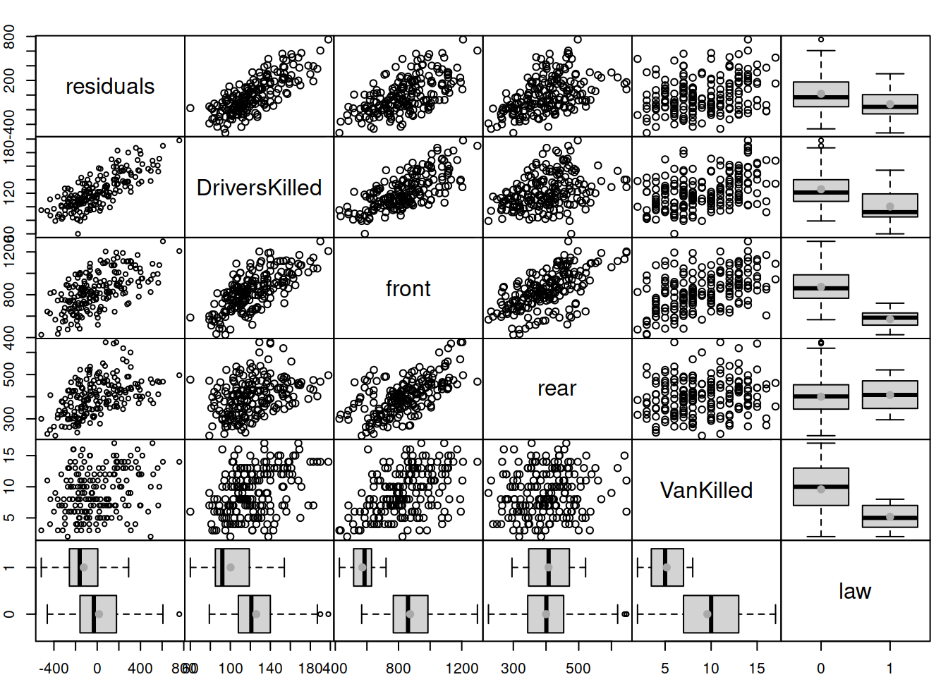
Figure 14.2: Spread plot for the residuals of model vs omitted variables.
The spread() function automatically detects the type of variable and based on that produces scatterplot/boxplot()/tableplot() between them, making the final plot more readable. The plot in Figure 14.2 tells us that residuals are correlated with DriversKilled, front, rear, and law, so some of these variables can be added to the model to improve it. However, not all of them make sense in our model. For example, VanKilled might have a weak relation with drivers, but judging by the description should not be included in the model (this is a part of the drivers variable). Also, I would not add DriversKilled, as it seems not to drive the number of deaths and injuries (based on our understanding of the problem), but is just correlated with it for obvious reasons (DriversKilled is included in drivers). The variables front and rear should not be included in the model either, because they do not explain injuries and deaths of drivers, they are impacted by similar factors, and can be considered as output variables. So, only law can be safely added to the model, because it makes sense: the introduction of law should hopefully impact the number of casualties amongst drivers.
We can also calculate measures of association between these variables to get an idea of the strength of linear relations bewteen them:
## Associations:
## values:
##               residuals DriversKilled  front   rear VanKilled    law
## residuals        1.0000        0.7826 0.6121 0.4811    0.2751 0.1892
## DriversKilled    0.7826        1.0000 0.7068 0.3534    0.4070 0.3285
## front            0.6121        0.7068 1.0000 0.6202    0.4724 0.5624
## rear             0.4811        0.3534 0.6202 1.0000    0.1218 0.0291
## VanKilled        0.2751        0.4070 0.4724 0.1218    1.0000 0.3949
## law              0.1892        0.3285 0.5624 0.0291    0.3949 1.0000
##
## p-values:
##               residuals DriversKilled front   rear VanKilled    law
## residuals        0.0000             0     0 0.0000    0.0001 0.0086
## DriversKilled    0.0000             0     0 0.0000    0.0000 0.0000
## front            0.0000             0     0 0.0000    0.0000 0.0000
## rear             0.0000             0     0 0.0000    0.0925 0.6890
## VanKilled        0.0001             0     0 0.0925    0.0000 0.0000
## law              0.0086             0     0 0.6890    0.0000 0.0000
##
## types:
##               residuals DriversKilled front     rear      VanKilled law
## residuals     "none"    "pearson"     "pearson" "pearson" "pearson" "mcor"
## DriversKilled "pearson" "none"        "pearson" "pearson" "pearson" "mcor"
## front         "pearson" "pearson"     "none"    "pearson" "pearson" "mcor"
## rear          "pearson" "pearson"     "pearson" "none"    "pearson" "mcor"
## VanKilled     "pearson" "pearson"     "pearson" "pearson" "none"    "mcor"
## law           "mcor"    "mcor"        "mcor"    "mcor"    "mcor"    "none"
Technically speaking, the output of this function tells us that all variables are correlated with residuals and can be considered in the model. This is because p-values are lower than my favourite significance level of 1%, so we can reject the null hypothesis for each of the tests (which is that the respective parameter is equal to zero in the population). I would still prefer not to add DriversKilled, VanKilled, front, and rear variables in the model for the reasons explained earlier, but I would add law:
The model now fits the data differently (Figure 14.3):
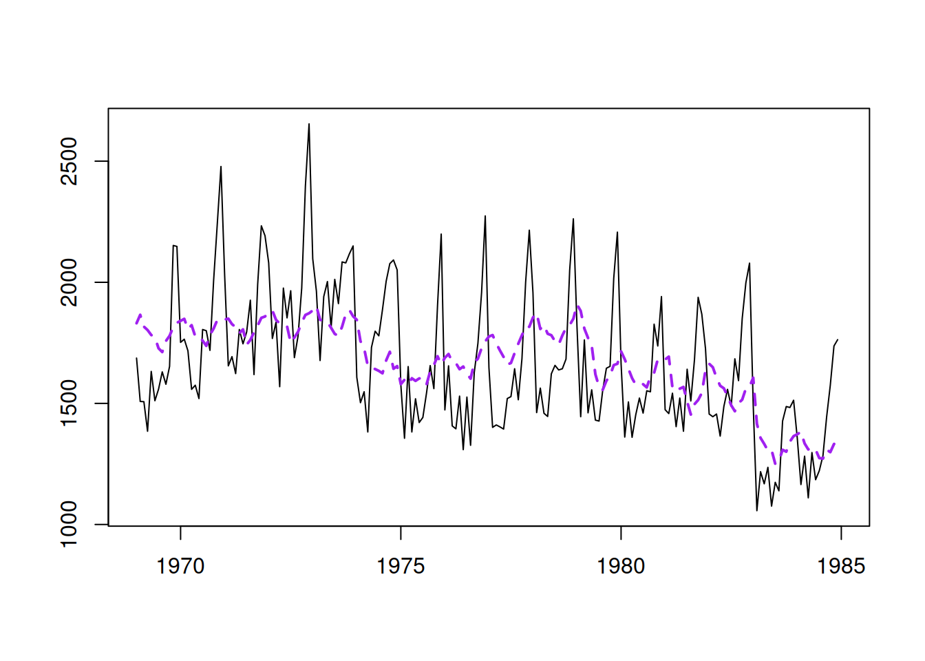
Figure 14.3: The data and the fitted values for the second model.
How can we know that we have not omitted any important variables in our new model? Unfortunately, there is no good way of knowing that. In general, we should use judgment to decide whether anything else is needed or not. But given that we deal with time series, we can analyse residuals over time and see if there is any structure left (Figure 14.4):
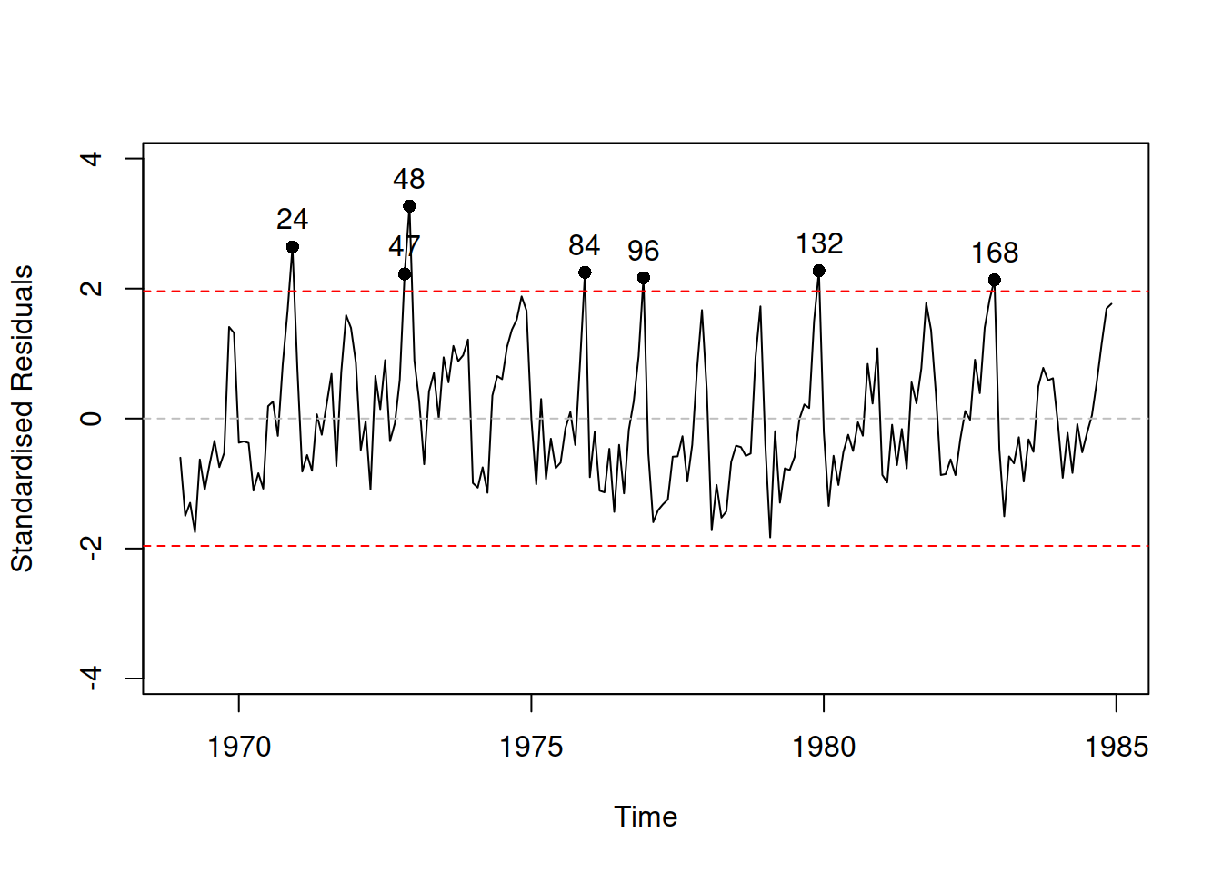
Figure 14.4: Standardised residuals vs time plot.
Plot in Figure 14.4 shows that the model has not captured seasonality correctly and that there is still some structure left in the residuals. In order to address this, we will add an ETS(A,N,A) element to the model, estimating ETSX instead of just regression:
We can then produce additional plots to do model diagnostics (Figue 14.5):
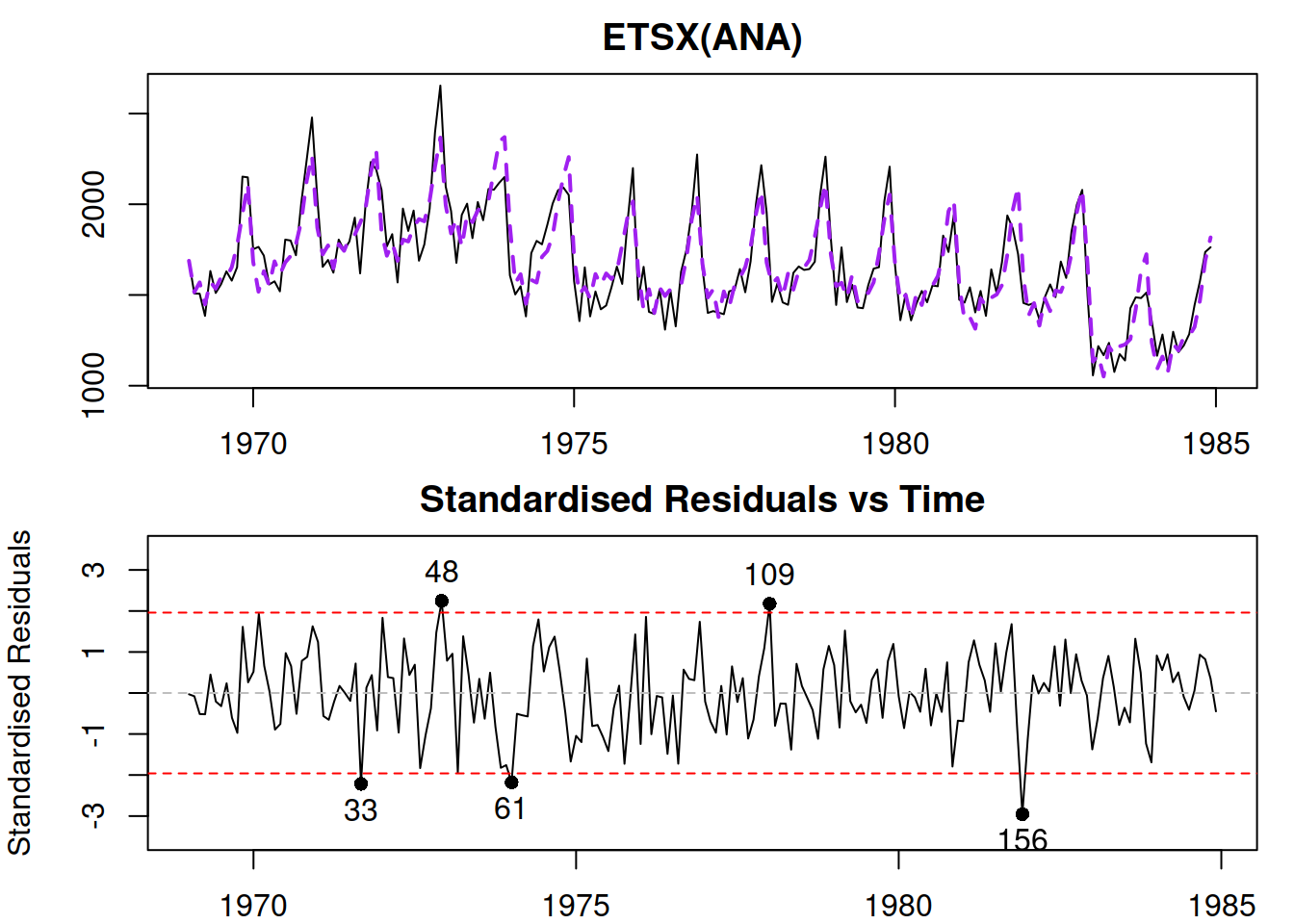
Figure 14.5: Diagnostic plots for Model 3.
In Figure 14.5, we do not see any apparent missing structure in the data and we do not have any additional variables to add. So, we can now move to the next step of diagnostics.