\( \newcommand{\mathbbm}[1]{\boldsymbol{\mathbf{#1}}} \)

12.5 Examples of application

12.5.1 ADAM ETS

We will use the taylor series from the forecast package to see how ADAM can be applied to high-frequency data. This is half-hourly electricity demand in England and Wales from Monday 5th June 2000 to Sunday 27th August 2000, used in Taylor (2003b).

library(zoo)
y <- zoo(forecast::taylor,
         order.by=as.POSIXct("2000/06/05")+
           (c(1:length(forecast::taylor))-1)*60*30)
plot(y)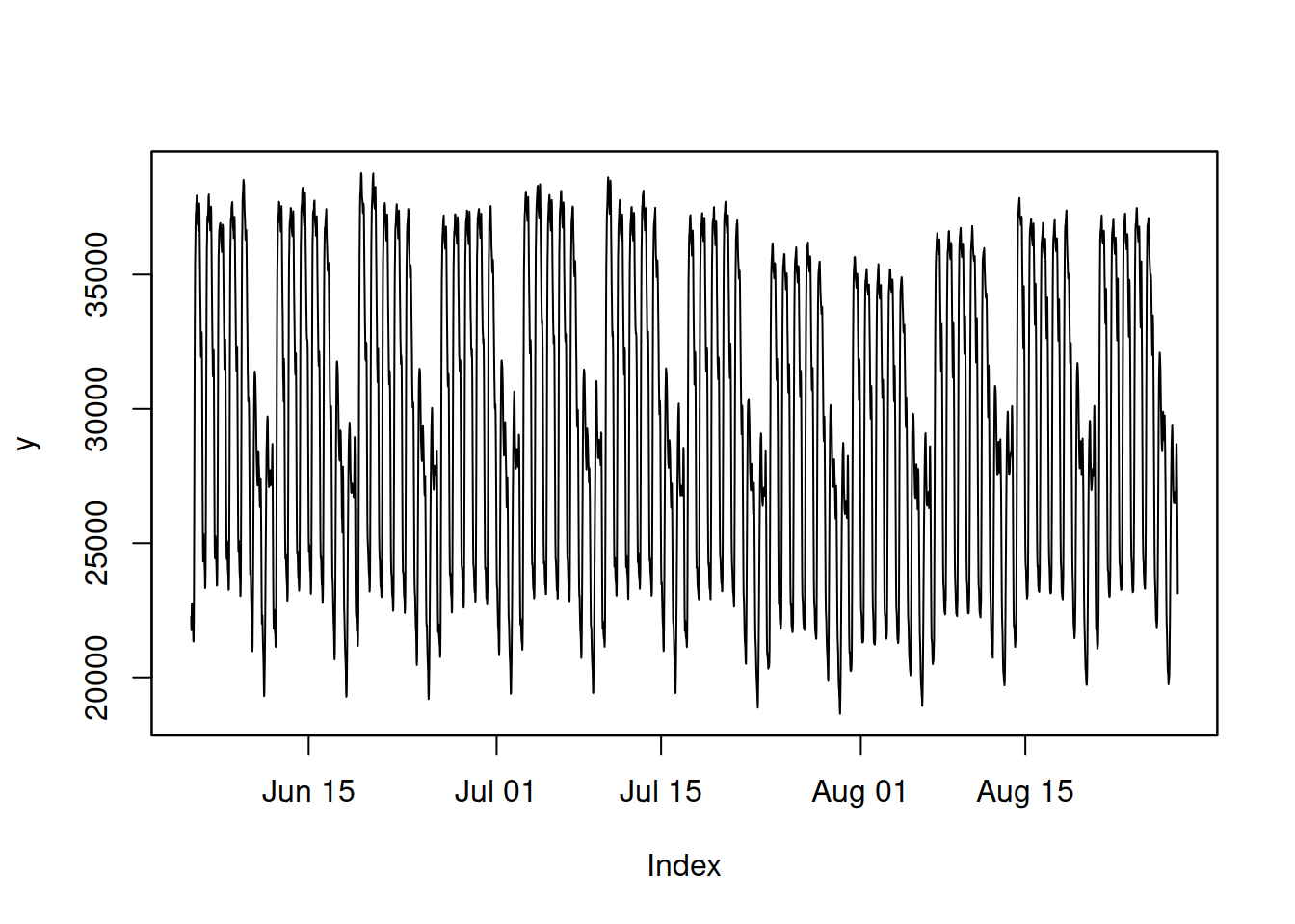

Figure 12.1: Half-hourly electricity demand in England and Wales.

The series in Figure 12.1 does not exhibit an apparent trend but has two seasonal cycles: a half-hour of the day and a day of the week. Seasonality seems to be multiplicative because, with the reduction of the level of series, the amplitude of seasonality also reduces. We will try several different models and see how they compare. In all the cases below, we will use backcasting to initialise the model. We will use the last 336 observations (\(48 \times 7\)) as the holdout to see whether models perform adequately or not.

Remark. When we have data with DST or leap years (as discussed in Section 12.4), adam() will automatically correct the seasonal lags as long as your data contains specific dates (as zoo objects have, for example).

First, it is ADAM ETS(M,N,M) with lags=c(48,7*48):

adamETSMNM <- adam(y, "MNM", lags=c(1,48,336),
                   h=336, holdout=TRUE,
                   initial="back")
adamETSMNM

## Time elapsed: 0.5 seconds
## Model estimated using adam() function: ETS(MNM)[48, 336]
## Distribution assumed in the model: Gamma
## Loss function type: likelihood; Loss function value: 25682.88
## Persistence vector g:
##  alpha gamma1 gamma2 
## 0.1357 0.2813 0.2335 
## 
## Sample size: 3696
## Number of estimated parameters: 4
## Number of degrees of freedom: 3692
## Information criteria:
##      AIC     AICc      BIC     BICc 
## 51373.76 51373.77 51398.62 51398.66 
## 
## Forecast errors:
## ME: 625.221; MAE: 716.941; RMSE: 817.796
## sCE: 709.966%; Asymmetry: 90.4%; sMAE: 2.423%; sMSE: 0.076%
## MASE: 1.103; RMSSE: 0.867; rMAE: 0.107; rRMSE: 0.1

As we see from the output above, the model was constructed in 0.5 seconds. Notice that the seasonal smoothing parameters are relatively high in this model. For example, the second \(\gamma\) is equal to 0.2335, which means that the model adapts the seasonal profile to the data substantially (takes 23.35% of the error from the previous observation in it). Furthermore, the smoothing parameter \(\alpha\) is equal to 0.1357, which is also potentially too high, given that we have well-behaved data and that we deal with a multiplicative model. This might indicate that the model overfits the data. To see if this is the case, we can produce the plot of components over time (Figure 12.2).

plot(adamETSMNM, which=12)

Figure 12.2: Half-hourly electricity demand data decomposition according to ETS(M,N,M)[48,336].

As the plot in Figure 12.2 shows, the level of series repeats the seasonal pattern in the original data, although in a diminished way. In addition, the second seasonal component repeats the intra-day seasonality in it, although it is also reduced. Ideally, we want to have a smooth level component and for the second seasonal component not to have those spikes for half-hour of day seasonality.

Next, we can plot the fitted values and forecasts to see how the model performs overall (Figure 12.3).

plot(adamETSMNM, which=7)

Figure 12.3: The fit and the forecast of the ETS(M,N,M)[48,336] model on half-hourly electricity demand data.

As we see from Figure 12.3, the model fits the data well and produces reasonable forecasts. Given that it only took one second for the model estimation and construction, this model can be considered a good starting point. If we want to improve upon it, we can try one of the multistep estimators, for example, GTMSE (Subsection 11.3.3):

adamETSMNMGTMSE <- adam(y, "MNM", lags=c(1,48,336),
                        h=336, holdout=TRUE,
                        initial="back", loss="GTMSE")

The function will take more time due to complexity in the loss function calculation, but hopefully, it will produce more accurate forecasts due to the shrinkage of smoothing parameters:

adamETSMNMGTMSE

## Time elapsed: 23.06 seconds
## Model estimated using adam() function: ETS(MNM)[48, 336]
## Distribution assumed in the model: Normal
## Loss function type: GTMSE; Loss function value: -2648.698
## Persistence vector g:
##  alpha gamma1 gamma2 
## 0.0314 0.2604 0.1414 
## 
## Sample size: 3696
## Number of estimated parameters: 3
## Number of degrees of freedom: 3693
## Information criteria are unavailable for the chosen loss & distribution.
## 
## Forecast errors:
## ME: 216.71; MAE: 376.291; RMSE: 505.375
## sCE: 246.084%; Asymmetry: 63%; sMAE: 1.272%; sMSE: 0.029%
## MASE: 0.579; RMSSE: 0.535; rMAE: 0.056; rRMSE: 0.062

The smoothing parameters of the second model are closer to zero than in the first one, which might mean that it does not overfit the data as much. We can analyse the components of the second model by plotting them over time, similarly to how we did it for the previous model (Figure 12.4):

plot(adamETSMNMGTMSE, which=12)

Figure 12.4: Half-hourly electricity demand data decomposition according to ETS(M,N,M)[48,336] estimated with GTMSE.

The components on the plot in Figure 12.4 are still not ideal, but at least the level does not seem to contain the seasonality anymore. The seasonal components could still be improved if, for example, the initial seasonal indices were smoother (this applies especially to the seasonal component 2).

Comparing the accuracy of the two models, for example, using RMSSE, we can conclude that the one with GTMSE was more accurate than the one estimated using the conventional likelihood.

Another potential way of improvement for the model is the inclusion of an AR(1) term, as for example done by Taylor (2010). This might take more time than the first model, but could also lead to some improvements in the accuracy:

adamETSMNMAR <- adam(y, "MNM", lags=c(1,48,336),
                     initial="back", orders=c(1,0,0),
                     h=336, holdout=TRUE, maxeval=1000)

Estimating the ETS+ARIMA model is a complicated task because of the increase of dimensionality of the matrices in the transition equation. Still, by default, the number of iterations would be restricted by 160, which might not be enough to get to the minimum of the loss. This is why I increased the number of iterations in the example above to 1000 via maxeval=1000. If you want to get more feedback on how the optimisation has been carried out, you can ask the function to print details via print_level=41. This is how the output of the model looks:

adamETSMNMAR

## Time elapsed: 2.07 seconds
## Model estimated using adam() function: ETS(MNM)[48, 336]+ARIMA(1,0,0)
## Distribution assumed in the model: Gamma
## Loss function type: likelihood; Loss function value: 24108.2
## Persistence vector g:
##  alpha gamma1 gamma2 
## 0.1129 0.2342 0.3180 
## 
## ARMA parameters of the model:
## AR:
## phi1[1] 
##  0.6923 
## 
## Sample size: 3696
## Number of estimated parameters: 5
## Number of degrees of freedom: 3691
## Information criteria:
##      AIC     AICc      BIC     BICc 
## 48226.39 48226.41 48257.47 48257.54 
## 
## Forecast errors:
## ME: 257.38; MAE: 435.476; RMSE: 561.237
## sCE: 292.266%; Asymmetry: 67.2%; sMAE: 1.472%; sMSE: 0.036%
## MASE: 0.67; RMSSE: 0.595; rMAE: 0.065; rRMSE: 0.069

In this specific example, we see that the ADAM ETS(M,N,M)+AR(1) leads to a slight improvement in accuracy in comparison with the ADAM ETS(M,N,M) estimated using the conventional loss function (it also has a lower AICc), but cannot beat the one estimated using GTMSE. We could try other options in adam() to get further improvements in accuracy, but we do not aim to get the best model in this section. An interested reader is encouraged to do that on their own.

12.5.2 ADAM ETSX

Another option of dealing with multiple seasonalities, as discussed in Section 12.3, is the introduction of explanatory variables. We start with a static model that captures half-hours of the day via its seasonal component and days of week frequency via an explanatory variable. We will use the temporaldummy() function from the greybox package to create respective categorical variables. This function works better when the data contains proper time stamps and, for example, is of class zoo or xts. It becomes especially useful when dealing with DST and leap years (see Section 12.4) because it will encode the dummy variables based on dates, allowing us to sidestep the issue with changing frequency in the data.

x1 <- temporaldummy(y,type="day",of="week",factors=TRUE)
x2 <- temporaldummy(y,type="hour",of="day",factors=TRUE)
taylorData <- data.frame(y=y,x1=x1,x2=x2)

Now that we created the data with categorical variables, we can fit the ADAM ETSX model with dummy variables for days of the week and use complete backcasting for initialisation:

adamETSXMNN <- adam(taylorData, "MNN", h=336, holdout=TRUE,
                    initial="complete")

In the code above, the initialisation method leads to potentially biased estimates of parameters at the cost of a reduced computational time (see discussion in Section 11.4.1). Here is what we get as a result:

adamETSXMNN

## Time elapsed: 0.61 seconds
## Model estimated using adam() function: ETSX(MNN)
## Distribution assumed in the model: Gamma
## Loss function type: likelihood; Loss function value: 30155.54
## Persistence vector g (excluding xreg):
##  alpha 
## 0.6182 
## 
## Sample size: 3696
## Number of estimated parameters: 2
## Number of degrees of freedom: 3694
## Information criteria:
##      AIC     AICc      BIC     BICc 
## 60315.08 60315.09 60327.51 60327.53 
## 
## Forecast errors:
## ME: -1664.294; MAE: 1781.472; RMSE: 2070.321
## sCE: -1889.878%; Asymmetry: -92.3%; sMAE: 6.021%; sMSE: 0.49%
## MASE: 2.74; RMSSE: 2.194; rMAE: 0.266; rRMSE: 0.253

The resulting model produces biased forecasts (they are consistently higher than needed). This is mainly because the smoothing parameter \(\alpha\) is too high, and the model frequently changes the level. We can see that in the plot of the state (Figure 12.5):

plot(adamETSXMNN$states[,1], ylab="Level")

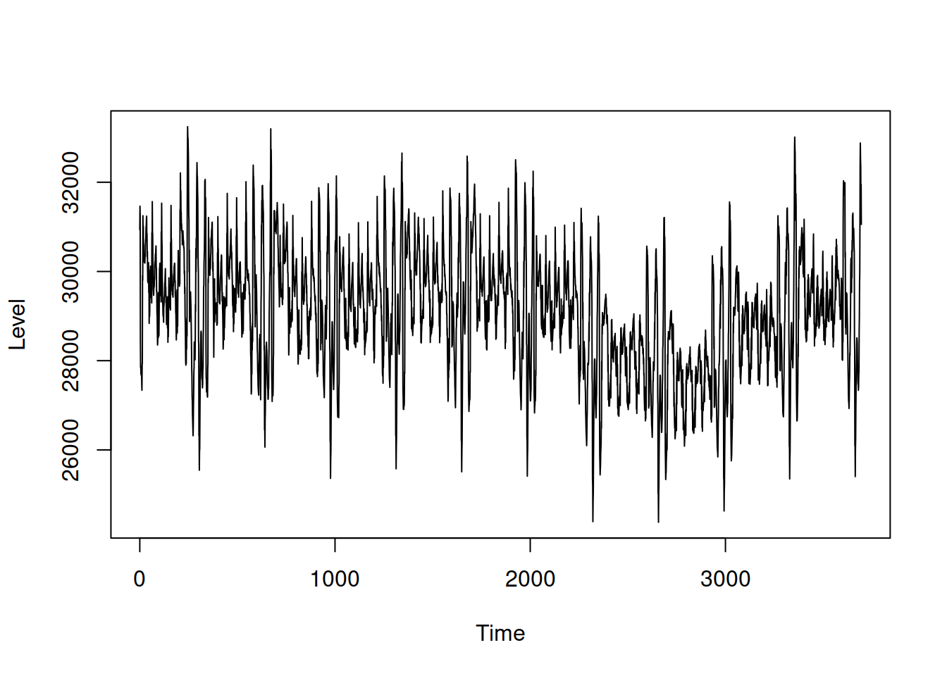
Figure 12.5: Plot of the level of the ETSX model.

As we see from Figure 12.5, the level component absorbs seasonality, which causes forecasting accuracy issues. However, the obtained value did not happen due to randomness – this is what the model does when seasonality is fixed and is not allowed to evolve. To reduce the model’s sensitivity, we can shrink the smoothing parameter using a multistep estimator (discussed in Section 11.3). But as discussed earlier, these estimators are typically slower than the conventional ones, so that they might take more computational time:

adamETSXMNNGTMSE <- adam(taylorData, "MNN",
                         h=336, holdout=TRUE,
                         initial="complete", loss="GTMSE")
adamETSXMNNGTMSE

## Time elapsed: 39.26 seconds
## Model estimated using adam() function: ETSX(MNN)
## Distribution assumed in the model: Normal
## Loss function type: GTMSE; Loss function value: -2044.705
## Persistence vector g (excluding xreg):
##  alpha 
## 0.0153 
## 
## Sample size: 3696
## Number of estimated parameters: 1
## Number of degrees of freedom: 3695
## Information criteria are unavailable for the chosen loss & distribution.
## 
## Forecast errors:
## ME: 105.462; MAE: 921.897; RMSE: 1204.967
## sCE: 119.757%; Asymmetry: 18%; sMAE: 3.116%; sMSE: 0.166%
## MASE: 1.418; RMSSE: 1.277; rMAE: 0.138; rRMSE: 0.147

While the model’s performance with GTMSE has improved due to the shrinkage of \(\alpha\) to zero, the seasonal states are still deterministic and do not adapt to the changes in data. We could adapt them via regressors="adapt", but then we would be constructing the ETS(M,N,M)[48,336] model but in a less efficient way. Alternatively, we could assume that one of the seasonal states is deterministic and, for example, construct the ETSX(M,N,M) model:

adamETSXMNMGTMSE <- adam(taylorData, "MNM", lags=48,
                         h=336, holdout=TRUE,
                         initial="complete", loss="GTMSE",
                         formula=y~x1)
adamETSXMNMGTMSE

## Time elapsed: 33.56 seconds
## Model estimated using adam() function: ETSX(MNM)
## Distribution assumed in the model: Normal
## Loss function type: GTMSE; Loss function value: -2082.17
## Persistence vector g (excluding xreg):
##  alpha  gamma 
## 0.0135 0.0769 
## 
## Sample size: 3696
## Number of estimated parameters: 2
## Number of degrees of freedom: 3694
## Information criteria are unavailable for the chosen loss & distribution.
## 
## Forecast errors:
## ME: 146.436; MAE: 830.332; RMSE: 1055.372
## sCE: 166.284%; Asymmetry: 27.1%; sMAE: 2.806%; sMSE: 0.127%
## MASE: 1.277; RMSSE: 1.118; rMAE: 0.124; rRMSE: 0.129

We can see an improvement compared to the previous model, so the seasonal states do change over time, which means that the deterministic seasonality is not appropriate in our example. However, it might be more suitable in some other cases, producing more accurate forecasts than the models assuming stochastic seasonality.

12.5.3 ADAM ARIMA

Another model we can try on this data is Multiple Seasonal ARIMA. We have not yet discussed the order selection mechanism for ARIMA, so I will construct a model based on my judgment. Keeping in mind that ETS(A,N,N) is equivalent to ARIMA(0,1,1) and that the changing seasonality in the ARIMA context can be modelled with seasonal differences, I will construct SARIMA(0,1,1)(0,1,1)\(_{336}\), skipping the frequencies for a half-hour of the day. Hopefully, this will suffice to model: (a) changing level of data; (b) changing seasonal amplitude. Here is how we can construct this model using adam():

adamARIMA <- adam(y, "NNN", lags=c(1,336), initial="back",
                  orders=list(i=c(1,1),ma=c(1,1)),
                  h=336, holdout=TRUE)
adamARIMA

## Time elapsed: 0.2 seconds
## Model estimated using adam() function: SARIMA(0,1,1)[1](0,1,1)[336]
## Distribution assumed in the model: Normal
## Loss function type: likelihood; Loss function value: 26098.77
## ARMA parameters of the model:
## MA:
##   theta1[1] theta1[336] 
##      0.5086     -0.1969 
## 
## Sample size: 3696
## Number of estimated parameters: 3
## Number of degrees of freedom: 3693
## Information criteria:
##      AIC     AICc      BIC     BICc 
## 52203.53 52203.54 52222.18 52222.20 
## 
## Forecast errors:
## ME: 49.076; MAE: 373.297; RMSE: 499.539
## sCE: 55.728%; Asymmetry: 18.5%; sMAE: 1.262%; sMSE: 0.029%
## MASE: 0.574; RMSSE: 0.529; rMAE: 0.056; rRMSE: 0.061

As we see from the output above, this model has the lowest RMSSE value among all models we tried. Furthermore, this model is directly comparable with ADAM ETS via information criteria, and as we can see, it is worse than ADAM ETS(M,N,M)+AR(1) and multiple seasonal ETS(M,N,M) in terms of AICc. One of potential ways of improving this model is to try a different distribution for the error term. To aid us in this task, we can produce a QQ-plot (see details in Section 14.8):

plot(adamARIMA, 6)

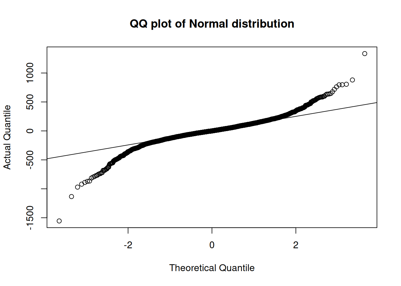
Figure 12.6: QQ plot of the ARIMA model with Normal distribution.

Figure 12.6 shows that the empirical distribution of residual has much fatter tails than in case of the normal distribution. Instead of trying to find the most suitable distribution (which can be done automatically as discussed in Chapter 15), I will fit the same ARIMA model, but with the Generalised Normal distribution:

adamARIMAGN <- adam(y, "NNN", lags=c(1,336), initial="back",
                    orders=list(i=c(1,1),ma=c(1,1)),
                    h=336, holdout=TRUE, distribution="dgnorm")
adamARIMAGN

## Time elapsed: 0.39 seconds
## Model estimated using adam() function: SARIMA(0,1,1)[1](0,1,1)[336]
## Distribution assumed in the model: Generalised Normal with shape=0.7511
## Loss function type: likelihood; Loss function value: 25145.3
## ARMA parameters of the model:
## MA:
##   theta1[1] theta1[336] 
##      0.2671     -0.1579 
## 
## Sample size: 3696
## Number of estimated parameters: 4
## Number of degrees of freedom: 3692
## Information criteria:
##      AIC     AICc      BIC     BICc 
## 50298.59 50298.60 50323.45 50323.50 
## 
## Forecast errors:
## ME: 75.822; MAE: 375.101; RMSE: 498.56
## sCE: 86.099%; Asymmetry: 25.7%; sMAE: 1.268%; sMSE: 0.028%
## MASE: 0.577; RMSSE: 0.528; rMAE: 0.056; rRMSE: 0.061

This model now has much lower AICc than the previous models and should have a better behaved residuals (an interested reader is encouraged to produce a QQ-plot similarly to how it was done above).

Figure 12.7 shows the fit and forecast from this model.

plot(adamARIMAGN, which=7)

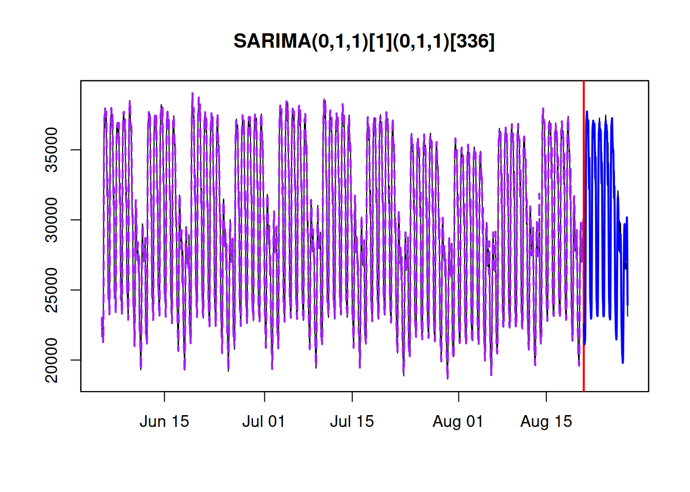
Figure 12.7: The fit and the forecast of the ARIMA(0,1,1)(0,1,1)\(_{336}\) model with Generalised Normal distribution on half-hourly electricity demand data.

We could analyse the residuals of this model further and iteratively test whether the addition of AR terms and a half-hour of day seasonality improves the model’s accuracy. We could also try ARIMA models with other distributions, compare them and select the most appropriate one or estimate the model using multistep losses. All of this can be done in adam(). The reader is encouraged to do this on their own.

References

• Taylor, J.W., 2010. Triple Seasonal Methods for Short-term Electricity Demand Forecasting. European Journal of Operational Research. 204, 139–152. https://doi.org/10.1016/j.ejor.2009.10.003

• Taylor, J.W., 2003b. Short-term Electricity Demand Forecasting Using Double Seasonal Exponential Smoothing. Journal of the Operational Research Society. 54, 799–805. https://doi.org/10.1057/palgrave.jors.2601589