16.5 Multi-scenarios for ADAM states
As discussed in Section 16.4, it is difficult to capture the impact of the uncertainty about the parameters on the states of the model and, as a result, difficult to take it into account on the forecasting stage. Furthermore, so far, we have only discussed pure additive models, for which it is at least possible to do some derivations. When it comes to models with multiplicative components, it becomes nearly impossible to demonstrate how the uncertainty propagates over time. To overcome these limitations, we developed (Svetunkov and Pritularga, 2023) a simulation-based approach (similar to the one discussed in Section 16.1) that relies on the selected model form.
The idea of the approach is to get the covariance matrix of the parameters of the selected model (see Section 16.2) and then generate \(n\) sets of parameters randomly from a Rectified Multivariate Normal distribution using the matrix and the values of estimated parameters. After that, the model is applied to the data with each generated parameters combination to get the states, fitted values, and residuals (simulation is done using the principles from Section 16.1). This way, we propagate the uncertainty about the parameters from the first observation to the last one. The final states can then be used to produce point forecasts and prediction intervals based on each set of parameters. These scenarios allow creating more adequate prediction intervals from the model and/or confidence intervals for the fitted values, states, and conditional expectations. All of this is done without any additional model assumptions and without any additional modelling steps, relying entirely on the estimated ADAM. This approach is computationally expensive, as it requires fitting all the \(n\) models to the data, however no estimation is needed. Furthermore, if the uncertainty about the model needs to be taken into account, then the combination of models can be used, as described in Section 15.4, where the approach from this section would be applied for each of the models in the pool before combining the point forecasts and prediction intervals with information criteria weights.
The smooth package has the method reapply() that implements this approach for adam() models. This works with ADAM ETS, ARIMA, regression, and any combination of the three. Here is an example in R with \(n=1000\):
# Estimate the model
adamETSAir <- adam(AirPassengers, "MMM", h=10, holdout=TRUE,
                   maxeval=16*100)
# Produce the multiple scenarios
adamETSAirReapply <- reapply(adamETSAir, nsim=1000)Remark. In the code above I have increased the number of iterations in the optimiser to \(k \times 100\), because I noticed that the default value does not allow reaching the maximum of the likelihood, and as a result the variances of parameters become too large. At the moment, there is no automated solution to this problem and \(k \times 100\) is a heuristic that can be used if a more precise optimum is required.
After producing the scenarios, we can plot them (see Figure 16.3).
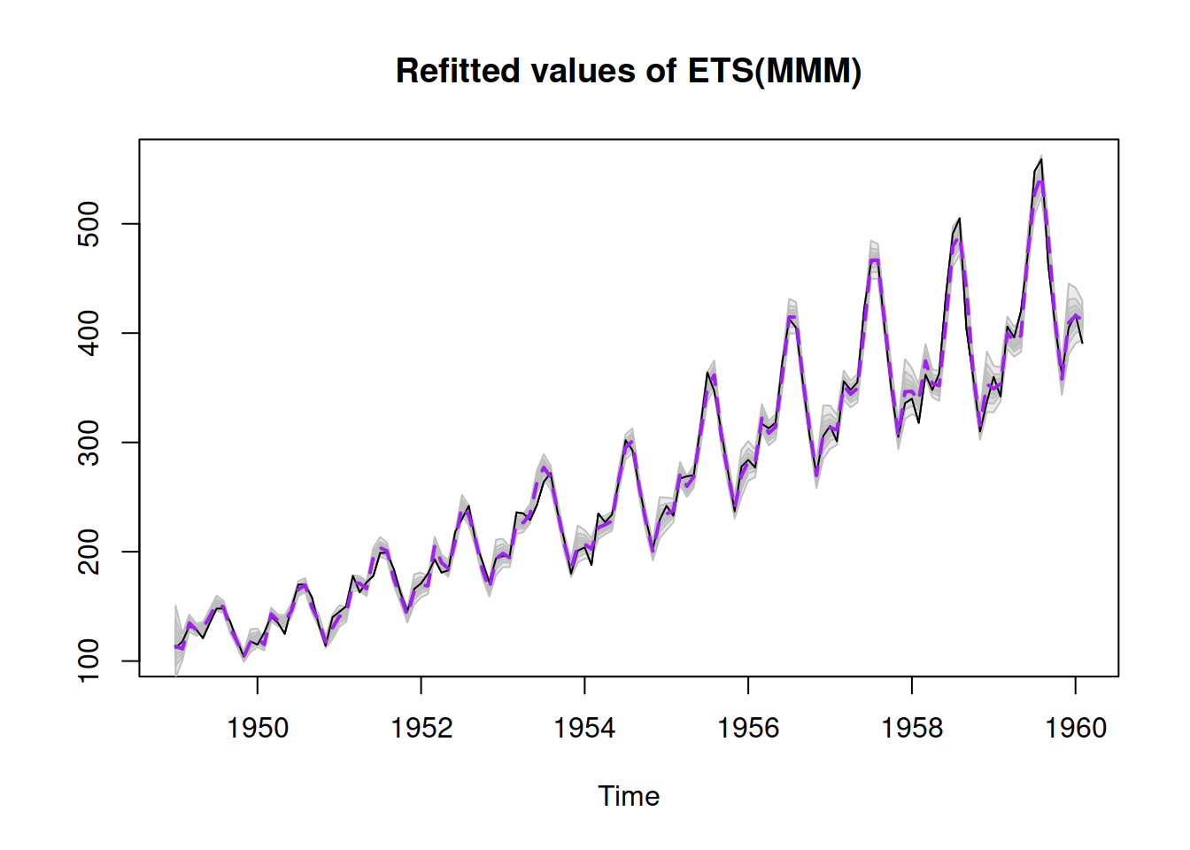
Figure 16.3: Refitted ADAM ETS(M,M,M) model on AirPassengers data.
Figure 16.3 demonstrates how the approach works on the example of AirPassengers data with an ETS(M,M,M) model. The grey areas around the fitted line show quantiles from the fitted values, forming confidence intervals of the width 95%, 80%, 60%, 40%, and 20%. They show how the fitted value would vary if the parameters would differ from the estimated ones. Notice that there was a warning about the covariance matrix of parameters, which typically appears if the optimal value of the loss function was not reached. If this happens, I would recommend tuning the optimiser (see Section 11.4).
The adamETSAirReapply object contains several variables, including:
adamETSAirReapply$states– the array of states of dimensions \(k \times (T+m) \times n\), where \(m\) is the maximum lag of the model, \(k\) is the number of components, and \(T\) is the sample size;adamETSAirReapply$refitted– fitted values produced from different parameters, dimensions \(T \times n\);adamETSAirReapply$transition– the array of transition matrices of the size \(k \times k \times n\);adamETSAirReapply$measurement– the array of measurement matrices of the size \((T+m) \times k \times n\);adamETSAirReapply$persistence– the persistence matrix of the size \(k \times n\);
The last three will contain the random parameters (smoothing, dampening, and AR/MA parameters), which is why they are provided together with the other values.
As mentioned earlier, ADAM ARIMA also supports this approach. Here is an example on an artificial, non-seasonal data, generated from ARIMA(0,1,1) (see Figure 16.4):
set.seed(41)
# Generate the data
y <- sim.ssarima(orders=list(i=1,ma=1), obs=120, MA=-0.7)
# Apply ADAM, then refit it and plot
adam(y$data, "NNN", h=10, holdout=TRUE,
     orders=c(0,1,1)) |>
    reapply() |>
    plot()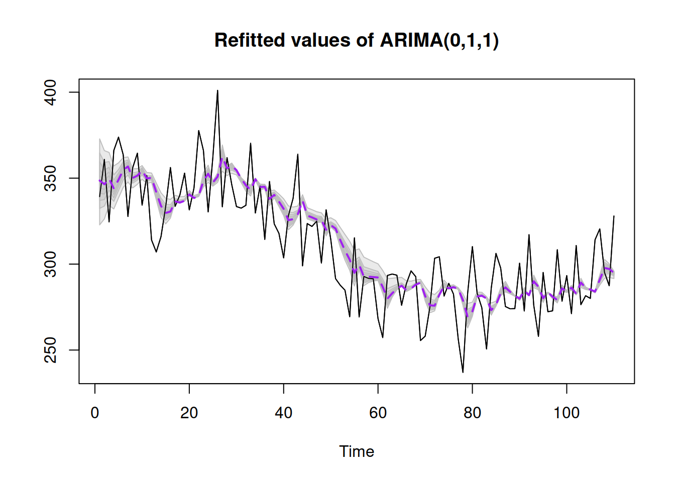
Figure 16.4: Refitted ADAM ARIMA(0,1,1) model on artificial data.
Note that the more complicated the fitted model is, the more difficult it is to optimise, and thus the more difficult it is to get accurate estimates of the covariance matrix of parameters. This might result in highly uncertain states and thus fitted values. The safer approach, in this case, is using bootstrap for the estimation of the covariance matrix, but this is more computationally expensive and would only work on longer time series. Here is how bootstrap can be used for the multi-scenarios in R (and Figure 16.5):
adam(y$data, "NNN", h=10, holdout=TRUE,
     orders=c(0,1,1)) |>
    reapply(bootstrap=TRUE, parallel=TRUE) |>
    plot()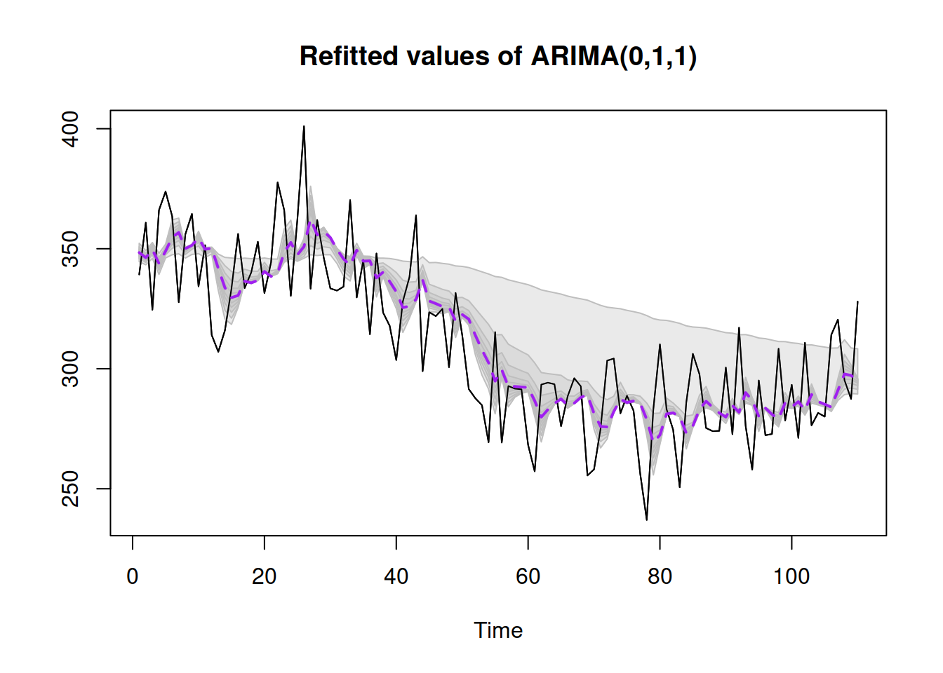
Figure 16.5: Refitted ADAM ARIMA(0,1,1) model on artificial data, bootstrapped covariance matrix.
The approach described in this section is still a work in progress. While it works in theory, there are computational difficulties with calculating the Hessian matrix in some situations. If the covariance matrix is not estimated accurately, it might contain high variances, leading to higher than needed uncertainty of the model. This might result in unreasonable confidence bounds and lead to extremely wide prediction intervals.