8.3 Box-Jenkins approach
Now that we are more or less familiar with the idea of ARIMA models, we can move to practicalities. As it might become apparent from the previous sections, one of the issues with the model is the identification of orders p, d, q, P\(_j\), D\(_j\), Q\(_j\) etc. Back in the 20th century, when computers were slow, this was a challenging task, so George Box and Gwilym Jenkins (Box and Jenkins, 1976) developed a methodology for identifying and estimating ARIMA models. While there are more efficient ways of order selection for ARIMA nowadays, some of their principles are still used in time series analysis and in forecasting. We briefly outline the idea in this section, not purporting to give a detailed explanation of the approach.
8.3.1 Identifying stationarity
Before doing any time series analysis, we need to make the data stationary, which is done via the differences in the context of ARIMA (Section 8.1.5). But before doing anything, we need to understand whether the data is stationary or not in the first place: over-differencing typically is harmful to the model and would lead to misspecification issues. At the same time, in the case of under-differencing, it might not be possible to identify the model correctly.
There are different ways of understanding whether the data is stationary or not. The simplest of them is just looking at the data: in some cases, it becomes apparent that the mean of the data changes or that there is a trend in the data, so the conclusion would be relatively straightforward. If it is not stationary, then taking differences and analysing the differenced data again would be the next step to ensure that the second differences are not needed.
The more formal approach would be to conduct statistical tests, such as ADF (the adf.test() from the tseries package) or KPSS (the kpss.test() from the tseries package). Note that they test different hypotheses:
- In the case of ADF, it is:
- H\(_0\): the data is not stationary;
- H\(_1\): the data is stationary;
- In the case of KPSS:
- H\(_0\): the data is stationary;
- H\(_1\): the data is not stationary.
I do not intent to discuss how the tests are conducted and what they imply in detail, and the interested reader is referred to the original papers of Dickey and Fuller (1979) and Kwiatkowski et al. (1992). It should suffice to say that ADF is based on estimating parameters of the AR model and then testing the hypothesis for those parameters, while KPSS includes the component of Random Walk in a model (with potential trend) and checks whether the variance of that component is zero or not. Both tests have their advantages and disadvantages and sometimes might contradict each other. No matter what test you choose, do not forget what testing a statistical hypothesis means (see, for example, Section 8.1 of Svetunkov and Yusupova, 2025): if you fail to reject H\(_0\), it does not mean that it is true.
Remark. Even if you select the test-based approach, the procedure should still be iterative: test the hypothesis, take differences if needed, test the hypothesis again, etc. This way, we can determine the order of differences I(d).
When you work with seasonal data, the situation becomes more complicated. Yes, you can probably spot seasonality by visualising the data, but it is not easy to conclude whether the seasonal differences are needed. In this case, the Canova-Hansen test (the ch.test() in the uroot package) can be used to formally test the hypothesis similar to the one in the KPSS test, but applied to the seasonal differences.
Only after making sure that the data is stationary can we move to the identification of AR and MA orders.
8.3.2 Autocorrelation function (ACF)
At the core of the Box-Jenkins approach, lies the idea of autocorrelation and partial autocorrelation functions. Autocorrelation is the correlation (see Section 9.3 of Svetunkov and Yusupova, 2025) of a variable with itself from a different period of time. Here is an example of an autocorrelation coefficient for lag 1: \[\begin{equation} \rho(1) = \frac{\sigma_{y_t,y_{t-1}}}{\sigma_{y_t}\sigma_{y_{t-1}}} = \frac{\sigma_{y_t,y_{t-1}}}{\sigma_{y_t}^2}, \tag{8.60} \end{equation}\] where \(\rho(1)\) is the “true” autocorrelation coefficient, \(\sigma_{y_t,y_{t-1}}\) is the covariance between \(y_t\) and \(y_{t-1}\), while \(\sigma_{y_t}\) and \(\sigma_{y_{t-1}}\) are the “true” standard deviations of \(y_t\) and \(y_{t-1}\). Note that \(\sigma_{y_t}=\sigma_{y_{t-1}}\), because we are talking about one and the same variable. This is why we can simplify the formula to get the one on the right-hand side of (8.60). The formula (8.60) corresponds to the classical correlation coefficient, so this interpretation is the same as for the classical one: the value of \(\rho(1)\) shows the closeness of the lagged relation to linear. If it is close to one, then this means that variable has a strong linear relation with itself on the previous observation. It obviously does not tell you anything about the causality, just shows a technical relation between variables, even if it is spurious in real life.
Using the formula (8.60), we can calculate the autocorrelation coefficients for other lags as well, just substituting \(y_{t-1}\) with \(y_{t-2}\), \(y_{t-3}\), \(\dots\), \(y_{t-\tau}\) etc. In a way, \(\rho(\tau)\) can be considered a function of a lag \(\tau\), which is called the “Autocorrelation function” (ACF). If we know the order of the ARIMA process we deal with, we can plot the values of ACF on the y-axis by changing the \(\tau\) on the x-axis. Box and Jenkins (1976) discuss different theoretical functions for several special cases of ARIMA, which we do not plan to repeat here fully. But, for example, they show that if you deal with an AR(1) process, then the \(\rho(1)=\phi_1\), \(\rho(2)=\phi_1^2\), etc. This can be seen on the example of \(\rho(1)\) by calculating the covariance for AR(1): \[\begin{equation} \begin{aligned} \sigma_{y_t,y_{t-1}} = & \mathrm{cov}(y_t,y_{t-1}) = \mathrm{cov}(\phi_1 y_{t-1} + \epsilon_t, y_{t-1}) = \\ & \mathrm{cov}(\phi_1 y_{t-1}, y_{t-1}) = \phi_1 \sigma_{y_t}^2 , \end{aligned} \tag{8.61} \end{equation}\] which when inserted in (8.60) leads to \(\rho(1)=\phi_1\). The ACF for AR(1) with a positive \(\phi_1\) will have the shape shown in Figure 8.14 (on the example of \(\phi_1=0.9\)).
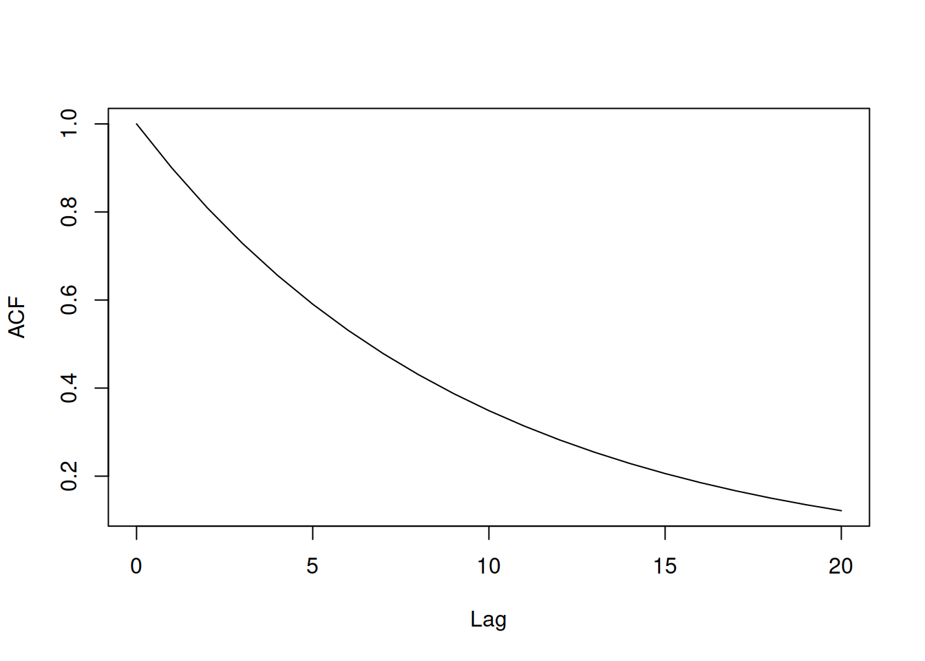
Figure 8.14: ACF for an AR(1) model.
Note that \(\rho(0)=1\) just because the value is correlated with itself, so lag 0 is typically dropped as not being useful. The declining shape of the ACF tells us that if \(y_t\) is correlated with \(y_{t-1}\), then the correlation between \(y_{t-1}\) and \(y_{t-2}\) will be exactly the same, also implying that \(y_{t}\) is somehow correlated with \(y_{t-2}\), even if there is no true relation between them. It is difficult to say anything for the AR process based on ACF exactly because of this temporal relation of the variable with itself.
On the other hand, ACF can be used to judge the order of an MA(q) process. For example, if we consider MA(1) (Section 8.1.2), then the \(\rho(1)\) will depend on the following covariance: \[\begin{equation} \begin{aligned} \sigma_{y_t,y_{t-1}} = & \mathrm{cov}(y_t,y_{t-1}) = \mathrm{cov}(\theta_1 \epsilon_{t-1} + \epsilon_t, \theta_1 \epsilon_{t-2} + \epsilon_{t-1}) = \\ & \mathrm{cov}(\theta_1 \epsilon_{t-1}, \epsilon_{t-1}) = \theta_1 \sigma^2 , \end{aligned} \tag{8.62} \end{equation}\] where \(\sigma^2\) is the variance of the error term, which in case of MA(1) is equal to \(\sigma^2_{y_t}\), because E\((y_t)=0\). However, the covariance between the higher lags will be equal to zero for the pure MA(1) (given that the usual assumptions from Section 1.4.1 hold). Box and Jenkins (1976) showed that for the moving averages, ACF tells more about the order of the model than for the autoregressive one: ACF will drop rapidly right after the specific lag q for the MA(q) process.
When it comes to seasonal models, in the case of seasonal AR(P), ACF will decrease exponentially from season to season (e.g. you would see a decrease on lags 4, 8, 12, etc. for SAR(1) and \(m=4\)), while in case of seasonal MA(Q), ACF would drop abruptly, starting from the lag \((Q+1)m\) (so, the subsequent seasonal lag from the one that the process has, e.g. on lag 8, if we deal with SMA(1) with \(m=4\)).
8.3.3 Partial autocorrelation function (PACF)
The other instrument useful for time series analysis with respect to ARIMA is called “partial ACF”. The idea of this follows from ACF directly. As we have spotted, if the process we deal with follows AR(1), then \(\rho(2)=\phi_1^2\) just because of the temporal relation. In order to get rid of this temporal effect, when calculating the correlation between \(y_t\) and \(y_{t-2}\) we could remove the correlation \(\rho(1)\) in order to get the clean effect of \(y_{t-2}\) on \(y_t\). This type of correlation is called “partial”, denoting it as \(\varrho(\tau)\). There are different ways to do that. One of the simplest is to estimate the following regression model: \[\begin{equation} y_t = a_1 y_{t-1} + a_2 y_{t-2} + \dots + a_\tau y_{t-\tau} + \epsilon_t, \tag{8.63} \end{equation}\] where \(a_i\) is the parameter for the \(i\)-th lag of the model. In this regression, all the relations between \(y_t\) and \(y_{t-\tau}\) are captured separately, so the last parameter \(a_\tau\) is clean of all the temporal effects discussed above. We then can use the value \(\varrho(\tau) = a_\tau\) as the coefficient, showing this relation. In order to obtain the PACF, we would need to construct and estimate regressions (8.63) for each lag \(\tau=\{1, 2, \dots, p\}\) and get the respective parameters \(a_1\), \(a_2\), \(\dots\), \(a_p\), which would correspond to \(\varrho(1)\), \(\varrho(2)\), \(\dots\), \(\varrho(p)\).
Just to show what this implies, we consider calculating PACF for an AR(1) process. In this case, the true model is: \[\begin{equation*} y_t = \phi_1 y_{t-1} + \epsilon_t. \end{equation*}\] For the first lag we estimate exactly the same model, so that \(\varrho(1)=\phi_1\). For the second lag we estimate the model: \[\begin{equation*} y_t = a_1 y_{t-1} + a_2 y_{t-2} + \epsilon_t. \end{equation*}\] But we know that for AR(1), \(a_2=0\), so when estimated in population, this would result in \(\varrho(2)=0\) (in the case of a sample, this would be a value very close to zero). If we continue with other lags, we will come to the same conclusion: for all lags \(\tau>1\) for the AR(1), we will have \(\varrho(\tau)=0\). This is one of the properties of PACF: if we deal with an AR(p) process, then PACF drops rapidly to zero right after the lag \(p\).
When it comes to the MA(q) process, PACF behaves differently. In order to understand how it would behave, we take an example of an MA(1) model, which is formulated as: \[\begin{equation*} y_t = \theta_1 \epsilon_{t-1} + \epsilon_t. \end{equation*}\] As it was discussed in Section 8.1.7, the MA process can be also represented as an infinite AR (see (8.36) for derivation): \[\begin{equation*} y_t = \sum_{j=1}^\infty -1^{j-1} \theta_1^j y_{t-j} + \epsilon_t. \end{equation*}\] If we construct and estimate the regression (8.63) for any lag \(\tau\) for such a process we will get \(\varrho(\tau)=-1^{\tau-1} \theta_1^\tau\). This would correspond to the exponentially decreasing curve (if the parameter \(\theta_1\) is positive, this will be an alternating series of values), similar to the one we have seen for the AR(1) and ACF. More generally, PACF will decline exponentially for an MA(q) process, starting from the \(\varrho(q)=\theta_q\).
When it comes to seasonal ARIMA models, the behaviour of PACF would resemble one of the non-seasonal ones, but with lags, multiple to the seasonality \(m\). e.g., for the SAR(1) process with \(m=4\), the \(\varrho(4)=\phi_{4,1}\), while \(\varrho(8)=0\).
8.3.4 Summary
Summarising the discussions in this section, we can conclude that:
- For an AR(p) process, ACF will decrease either exponentially or alternatingly (depending on the parameters’ values), starting from the lag \(p\);
- For an AR(p) process, PACF will drop abruptly right after the lag \(p\);
- For an MA(q) process, ACF will drop abruptly right after the lag \(q\);
- For an MA(q) process, PACF will decline either exponentially or alternatingly (based on the specific values of parameters), starting from the lag \(q\).
These rules are tempting to use when determining the appropriate order of the ARMA model. This is what Box and Jenkins (1976) propose to do, but in an iterative way, analysing the ACF/PACF of residuals of models obtained on previous steps. The authors also recommend identifying the seasonal orders before moving to the non-seasonal ones.
However, these rules are not necessarily bi-directional and might not work in practice, e.g. if we deal with MA(q), ACF drops abruptly right after the lag q, but if ACF drops abruptly after the lag q, then this does not necessarily mean that we deal with MA(q). The former follows directly from the assumed “true” model, while the latter refers to the identification of the model on the data, and there can be different reasons for the ACF to behave in the way it does. The logic here is similar to the following:
Example 8.1 All birds have wings. Sarah has wings. Thus, Sarah is a bird.
Here is Sarah:
Figure 8.15: Sarah by Yegor Kamelev.
This slight discrepancy led to issues in ARIMA identification over the years. We now understand that we should not rely entirely on the Box-Jenkins approach when identifying ARIMA orders. There are more appropriate methods for order selection, which can be used in the context of ARIMA (see, for example, Hyndman and Khandakar, 2008), and we will discuss some of them in Chapter 15. Still, ACF and PACF could be helpful in diagnostics. They might show you whether anything important is missing in the model. But they should not be used on their own. They are helpful together with other additional instruments (see discussion in Section 14.5).
8.3.5 Examples of ACF/PACF for several ARMA processes
Building upon the behaviours of ACF/PACF for AR and MA processes, we consider several examples of data generated from AR/MA. This might provide some guidelines of how the orders of ARMA can be identified in practice and show how challenging this is in some situations.
Figure 8.16 shows the plot of the data and ACF/PACF for an AR(1) process with \(\phi_1=0.9\). As discussed earlier, the ACF in this case declines exponentially, starting from lag 1, while the PACF drops right after the lag 1. The plot also shows how the fitted values and the forecast would look like if the order of the model was correctly selected and the parameters were known.
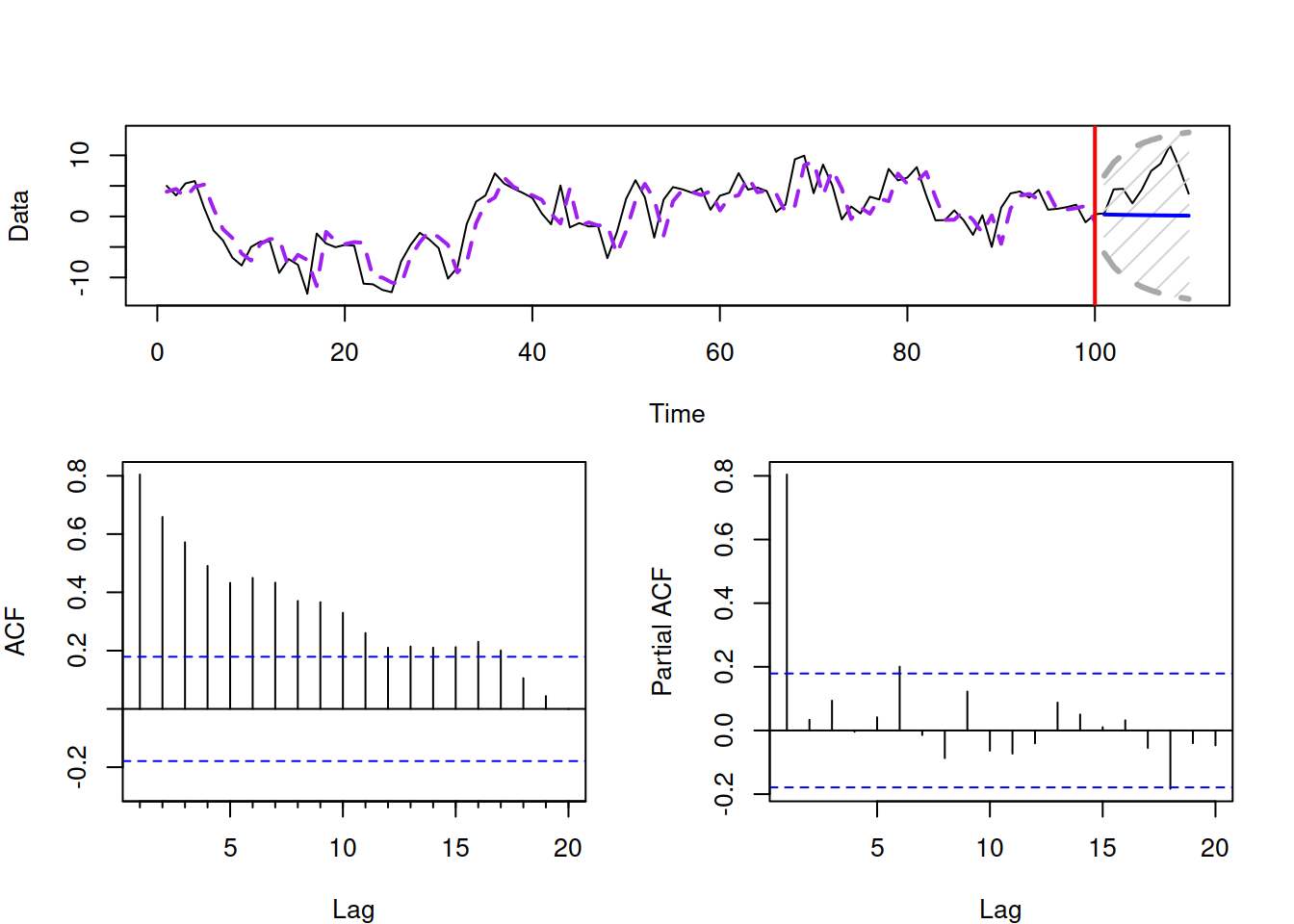
Figure 8.16: AR(1) process with \(\phi_1=0.9\).
Remark. You might notice that there are some values of the PACF lying outside the standard 95% confidence bounds in the plots above. This does not mean that we need to include the respective AR elements (AR(6) and AR(18)), because, by the definition of confidence interval, we can expect 5% of coefficients of correlation to lie outside the bounds, so we can ignore them.
A similar idea is shown in Figure 8.17 for an AR(2) process with \(\phi_1=0.9\) and \(\phi_2=-0.4\). In the Figure, the ACF oscillates slightly around the origin, while the PACF drops to zero right after the lag 2. These are the characteristics that we have discussed earlier in this section.
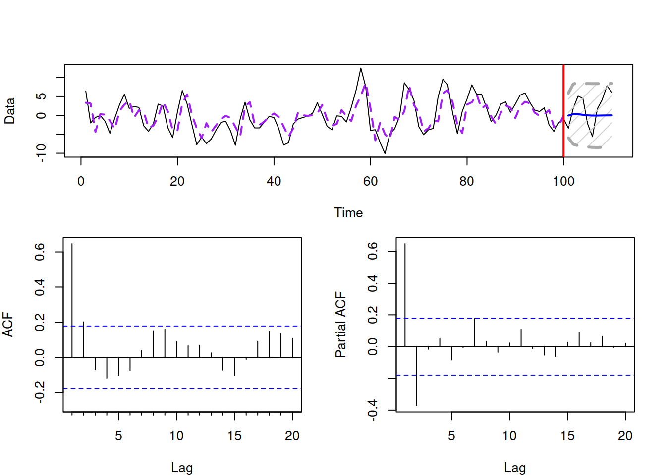
Figure 8.17: AR(2) process with \(\phi_1=0.9\) and \(\phi_2=-0.4\).
Similar plots but with different behaviours of ACF and PACF can be shown for MA(1) and MA(2) processes. Figure 8.18 shows how the MA(2) process looks like with \(\theta_1=-0.9\) and \(\theta_2=0.8\). As we can see, the correct diagnostics of the MA order in this case is already challenging: while the ACF drops to zero after lag 2, the PACF seems to contain some values outside of the interval on lags 3 and 4. So, using the Box and Jenkins (1976) approach, we would be choosing between an MA(2) and AR(1)/AR(4) models.
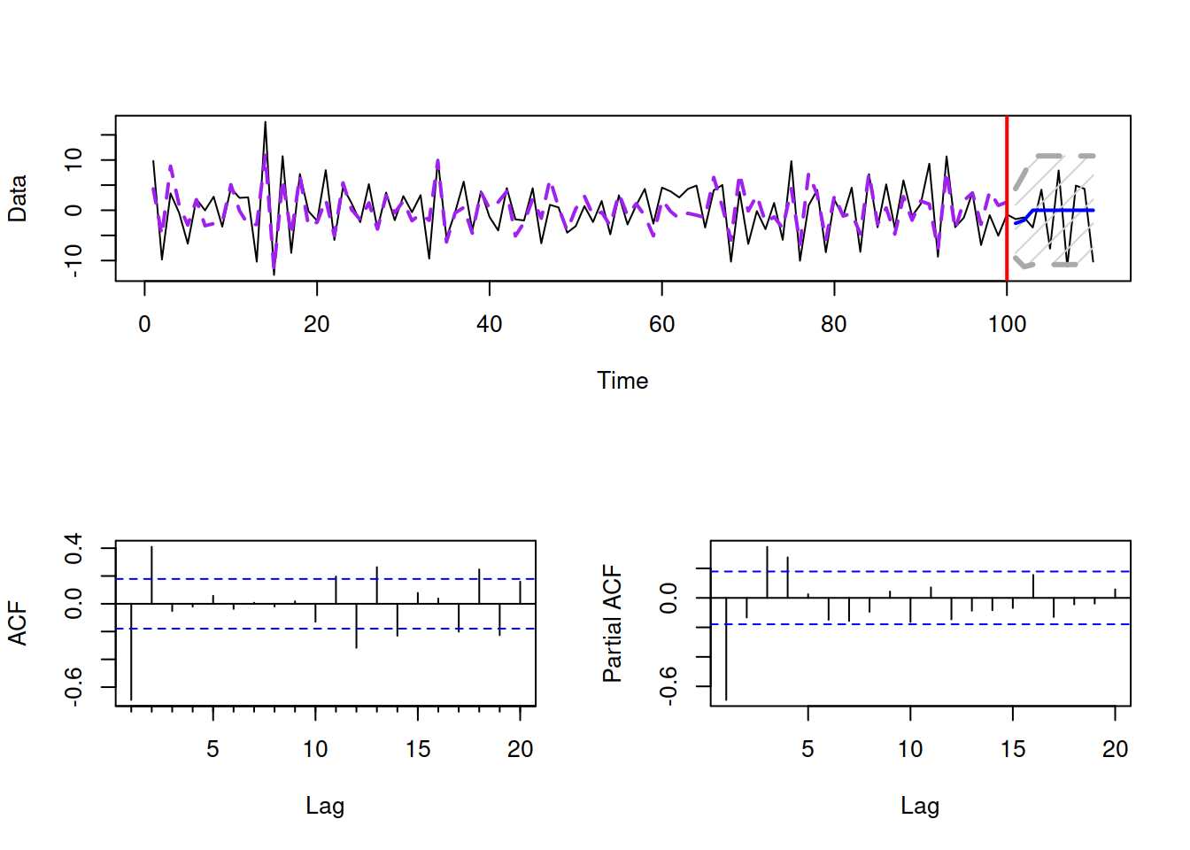
Figure 8.18: MA(2) process with \(\theta_1=-0.9\) and \(\theta_2=0.8\).
To make things even more complicated, we present similar plots for an ARMA(2,2) model in Figure 8.19.
Figure 8.19: ARMA(2,2) process with \(\phi_1=0.9, \phi_2=-0.4\), \(\theta_1=-0.9\) and \(\theta_2=0.8\).
Based on the ACF/PACF in Figure 8.19, we can conclude that the process is not fundamentally distinguishable from AR(2) and/or MA(2). In order to correctly identify the order in this situation, Box and Jenkins (1976) recommend doing the identification sequentially, by fitting an AR model, then analysing the residuals and selecting an appropriate MA order. Still, even this iterative process is challenging and does not guarantee that the correct order will be selected. This is one of the reasons why modern ARIMA order selection methods do not fully rely on the Box-Jenkins approach and involve selection based on information criteria Svetunkov and Boylan (2020).