3.2 Classical Seasonal Decomposition
3.2.1 How to do?
One of the classical textbook methods for decomposing the time series into unobservable components is “Classical Seasonal Decomposition” (Persons, 1919). It assumes either a pure additive or pure multiplicative model, is done using Centred Moving Averages (CMA), and is focused on splitting the data into components, not on forecasting. The idea of the method can be summarised in the following steps:
- Decide which of the models to use based on the type of seasonality in the data: additive (3.1) or multiplicative (3.2);
- Smooth the data using a CMA of order equal to the periodicity of the data \(m\). If \(m\) is an odd number then the formula is: \[\begin{equation} d_t = \frac{1}{m}\sum_{i=-(m-1)/2}^{(m-1)/2} y_{t+i}, \tag{3.4} \end{equation}\] which means that, for example, the value of \(d_t\) on Thursday is the average of all the actual values from Monday to Sunday. If \(m\) is an even number then a different weighting scheme is typically used, involving the inclusion of an additional value: \[\begin{equation} d_t = \frac{1}{m}\left(\frac{1}{2}\left(y_{t+(m-1)/2}+y_{t-(m-1)/2}\right) + \sum_{i=-(m-2)/2}^{(m-2)/2} y_{t+i}\right), \tag{3.5} \end{equation}\] which means that we use half of December of the previous year and half of December of the current year to calculate the CMA in June. The values \(d_t\) are placed in the middle of the window going through the series (e.g. as above, on Thursday, the average will contain values from Monday to Sunday).
The resulting series is deseasonalised. This is because when we average (e.g. sales in a year) we automatically remove the potential seasonality, which can be observed each period individually. A drawback of using CMA is that we inevitably lose \(\frac{m}{2}\) observations at the beginning and the end of the series.
In R, the ma() function from the forecast package implements CMA.
- De-trend the data:
- For the additive decomposition, this is done using: \({y^\prime}_t = y_t -d_t\);
- For the multiplicative decomposition, it is: \({y^\prime}_t = \frac{y_t}{d_t}\);
After that the series will only contain the residuals together with the seasonal component (if the data is seasonal).
If the data is seasonal, the average value for each period is calculated based on the de-trended series, e.g. we produce average seasonal indices for each January, February, etc. This will give us the set of seasonal indices \(s_t\). If the data is non-seasonal, we skip this step;
Calculate the residuals based on what you assume in the model:
- additive seasonality: \(e_t = y_t -d_t -s_t\);
- multiplicative seasonality: \(e_t = \frac{y_t}{d_t s_t}\);
- no seasonality: \(e_t = {y^\prime}_t\).
After doing steps (1) – (5), we will obtain several variables containing the components of a time series: \(s_t\), \(d_t\), and \(e_t\).
Remark. The functions in R typically allow selecting between additive and multiplicative seasonality. There is no option for “none”, and so even if the data is not seasonal, you will nonetheless get values for \(s_t\) in the output. Also, notice that the classical decomposition assumes that there is a deseasonalised series \(d_t\) but does not make any further split of this variable into level \(l_t\) and trend \(b_t\).
3.2.2 A couple of examples
An example of the classical decomposition in R is the decompose() function from the stats package. Here is an example with a pure multiplicative model and AirPassengers data (Figure 3.5).
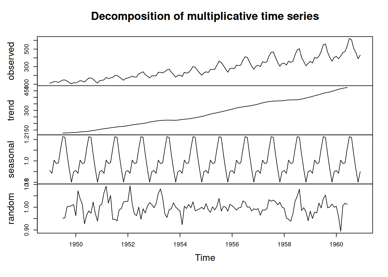
Figure 3.5: Decomposition of AirPassengers time series according to multiplicative model.
We can see from Figure 3.5 that the function has smoothed the original series and produced the seasonal indices. Note that the trend component has gaps at the beginning and the end. This is because the method relies on CMA (see above). Note also that the error term still contains some seasonal elements, which is a downside of such a simple decomposition procedure. However, the lack of precision in this method is compensated for by the simplicity and speed of calculation. Note again that the trend component in the decompose() function is in fact \(d_t = l_{t}+b_{t}\).
Figure 3.6 shows an example of decomposition of the non-seasonal data (we assume the pure additive model in this example).
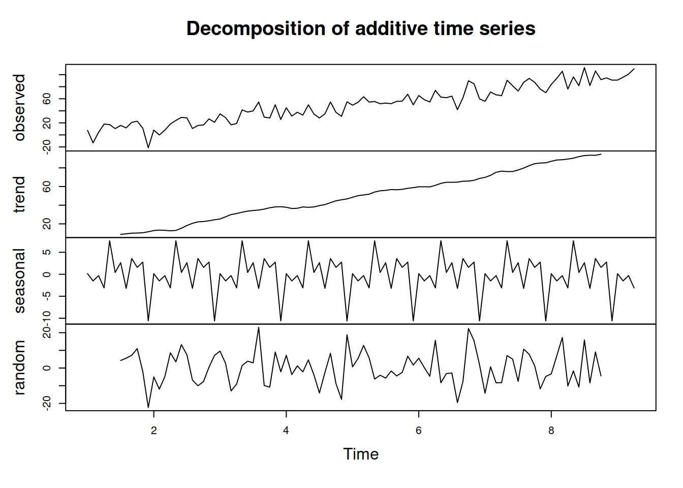
Figure 3.6: Decomposition of AirPassengers time series according to the additive model.
As we can see from Figure 3.6, the original data is not seasonal, but the decomposition assumes that it is and proceeds with the default approach, returning a seasonal component. You get what you ask for.
3.2.3 Multiple seasonal decomposition
A simple extension to the classical decomposition explained in Subsection 3.2.1 is the decomposition of data with multiple seasonal frequencies. In that case we need to use several CMAs and apply them sequentially to get rid of seasonaliities starting from the lower values and moving to the higher ones. This is better explained with an example of half-hourly data with two seasonal patterns: 48 half-hours per day and 336 (\(48 \times 7\)) half-hours per week. Assuming the pure multiplicative model, the decomposition procedure can be summarised as:
- Smooth the data:
- Use with CMA(48). This way we get rid of the lower level frequency and obtain the smooth pattern for the higher seasonal frequency of 336, \(d_{1,t}\);
- Smooth the same actual values with CMA(336). This way we get rid of both seasonal patterns and extract the trend, \(d_{2,t}\);
- Extract seasonal patterns:
- Divide the actual values by \(d_{1,t}\) to get seasonal indices for half-hours of day: \(y^\prime_{1,t}=\frac{y_t}{d_{1,t}}\);
- Divide \(d_{1,t}\) by \(d_{2,t}\) to get seasonal indices for half-hours of week: \(y^\prime_{2,t}=\frac{d_{1,t}}{d_{2,t}}\);
- Get seasonal indices:
- Average out the values of \(y^\prime_{1,t}\) for each period to get seasonal indices for half-hours of day \(s_{1,t}\);
- Do the same as (3.a) for each period of \(y^\prime_{2,t}\) to get half-hours of week \(s_{2,t}\);
- Finally, extract the residuals via: \(e_t = \frac{y_t}{d_{2,t} s_{1,t} s_{2,t}}\) and obtain the components of the decomposed series.
This procedure can be automated for data with more than two frequencies. The logic would be the same, we would just need to introduce more sub-steps (c, d, e) for each of the steps above (1, 2, 3). The procedure described above is implemented in the msdecompose() function from the smooth package. Here is how it works on the half-hourly data (from Taylor, 2003a) provided in the taylor object from the forecast package (Figure 3.7):
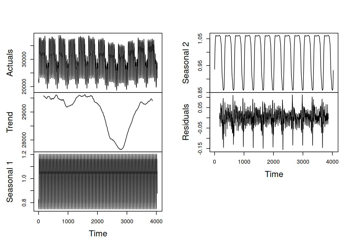
Figure 3.7: Decomposition of half-hourly electricity demand series according to the multiple seasonal classical decomposition.
The main limitation of this approach (similar to the conventional decomposition) is that it assumes that the seasonality does not evolve over time. This is a serious limitation if the seasonality needs to be used in forecasting. However, the procedure is simple and fast, and can be used as a starting point for the estimation of more complicated models (see, for example, Section 12.1).
3.2.4 Other decomposition techniques
There are other techniques that decompose series into error, trend, and seasonal components but make different assumptions about each component. The general procedure, however, always remains the same:
- Smooth the original series;
- Extract the seasonal components;
- Smooth them out.
The methods differ in the smoother they use (e.g. LOESS uses a bisquare function instead of CMA), and in some cases, multiple rounds of smoothing are performed to make sure that the components are split correctly.
There are many functions in R that implement seasonal decomposition. Here is a small selection:
decomp()from thetsutilspackage does classical decomposition and fills in the tail and head of the smoothed trend with forecasts from Exponential Smoothing;stl()from thestatspackage uses a different approach – seasonal decomposition via LOESS. It is an iterative algorithm that smooths the states and allows them to evolve over time. So, for example, the seasonal component in STL can change;mstl()from theforecastpackage does the STL for data with several seasonalities.
3.2.5 “Why bother?”
“Why decompose?” you may wonder at this point. Understanding the idea behind decomposition and how to perform it helps with the understanding of ETS, which relies on it. From a practical point of view, it can be helpful if you want to see if there is a trend in the data and whether the residuals contain outliers or not. It will not show you whether the data is seasonal or not as the seasonality is assumed in the decomposition (I stress this because many students think otherwise). Additionally, when seasonality cannot be added to a particular model under consideration, decomposing the series, predicting the trend, and then reseasonalising can be a viable solution. Finally, the values from the decomposition can be used as starting points for the estimation of components in ETS or other dynamic models relying on the error-trend-seasonality.