4.1 ETS taxonomy
Building on the idea of time series components (from Section 3.1), we can move to the ETS taxonomy. ETS stands for “Error-Trend-Seasonality” and defines how specifically the components interact with each other. Based on the type of error, trend, and seasonality, Pegels (1969) proposed a taxonomy, which was then developed further by Hyndman et al. (2002) and refined by Hyndman et al. (2008). According to this taxonomy, error, trend, and seasonality can be:
- Error: “Additive” (A), or “Multiplicative” (M);
- Trend: “None” (N), or “Additive” (A), or “Additive damped” (Ad), or “Multiplicative” (M), or “Multiplicative damped” (Md);
- Seasonality: “None” (N), or “Additive” (A), or “Multiplicative” (M).
In this taxonomy, the model (3.1) is denoted as ETS(A,A,A) while the model (3.2) is denoted as ETS(M,M,M), and (3.3) is ETS(M,A,M).
The components in the ETS taxonomy have clear interpretations: level shows average value per time period, trend reflects the change in the value, while seasonality corresponds to periodic fluctuations (e.g. increase in sales each January). Based on the the types of the components above, it is theoretically possible to devise 30 ETS models with different types of error, trend, and seasonality. Figure 4.1 shows examples of different time series with deterministic (they do not change over time) level, trend, seasonality, and with the additive error term.
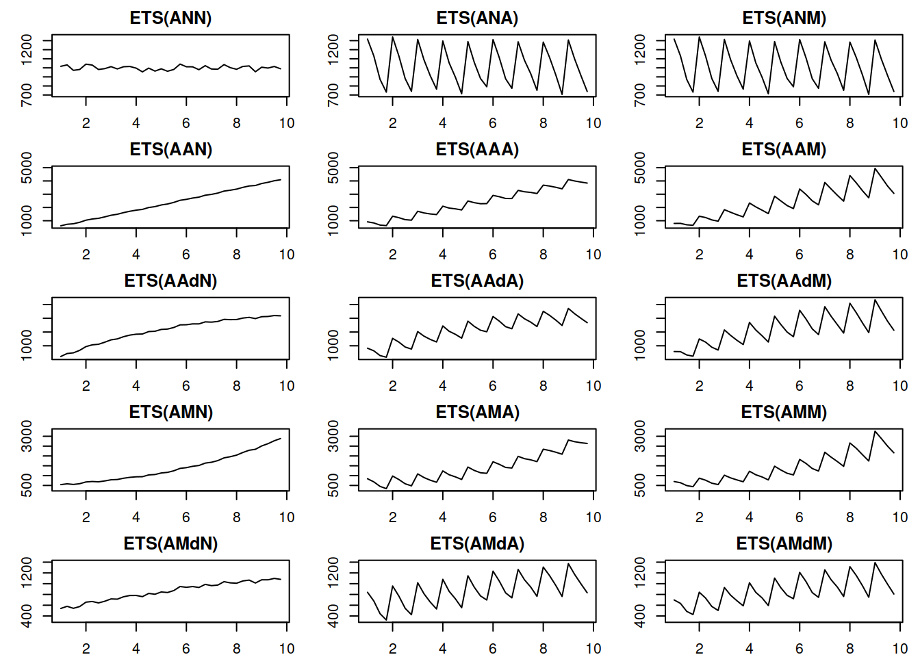
Figure 4.1: Time series corresponding to the additive error ETS models.
Things to note from the plots in Figure 4.1:
- When seasonality is multiplicative, its amplitude increases with the increase of the level of the data, while with additive seasonality, the amplitude is constant. Compare, for example, ETS(A,A,A) with ETS(A,A,M): for the former, the distance between the highest and the lowest points in the first year is roughly the same as in the last year. In the case of ETS(A,A,M) the distance increases with the increase in the level of series;
- When the trend is multiplicative, data exhibits exponential growth/decay;
- The damped trend slows down both additive and multiplicative trends;
- It is practically impossible to distinguish additive and multiplicative seasonality if the level of series does not change because the amplitude of seasonality will be constant in both cases (compare ETS(A,N,A) and ETS(A,N,M)).
Figure 4.2 demonstrates a similar plot for the multiplicative error models.
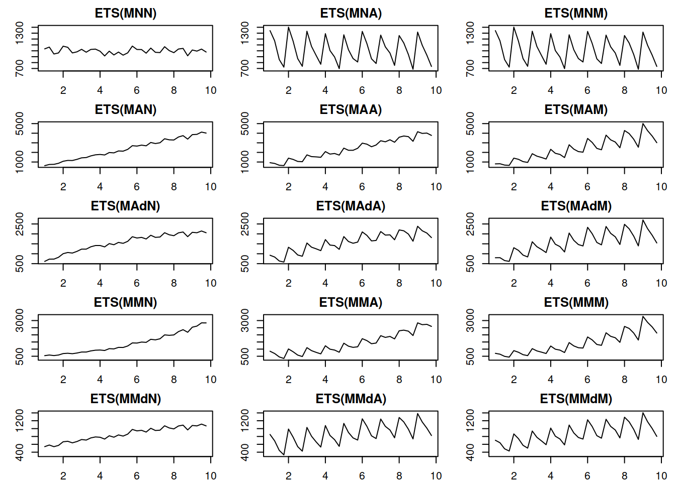
Figure 4.2: Time series corresponding to the multiplicative error ETS models.
The plots in Figure 4.2 show roughly the same idea as the additive case, the main difference being that the variance of the error increases with the increase of the level of the data – this becomes clearer on ETS(M,A,N) and ETS(M,M,N) data. This property is called heteroscedasticity in statistics, and Hyndman et al. (2008) argue that the main benefit of the multiplicative error models is in capturing this feature.
We will discuss the most important ETS family members in the following chapters. Note that not all the models in this taxonomy are sensible, and some are typically ignored entirely (this applies mainly to models with a mixture of additive and multiplicative components). ADAM implements the entire taxonomy, but we need to be aware of the potential issues with some of models, and we will discuss what to expect from them in different situations in the next chapters.