15.2 ARIMA order selection
While ETS has 30 models to choose from, ARIMA has thousands if not more. For example, selecting the non-seasonal ARIMA with/without constant restricting the orders with \(p \leq 3\), \(d \leq 2\), and \(q \leq 3\) leads to the combination of \(3 \times 2 \times 3 \times 2 = 36\) possible models. If we increase the possible orders to 5 or even more, we will need to go through hundreds of models. Adding the seasonal part increases this number by order of magnitude. Having several seasonal cycles, increases it further. This means that we cannot just test all possible ARIMA models and select the most appropriate one. We need to be smart in the selection process.
Hyndman and Khandakar (2008) developed an efficient mechanism of ARIMA order selection based on statistical tests (for stationarity and seasonality), reducing the number of models to test to a reasonable amount. Svetunkov and Boylan (2020) developed an alternative mechanism, relying purely on information criteria, which works well on seasonal data, but potentially may lead to models overfitting the data (this is implemented in the auto.ssarima() and auto.msarima() functions in the smooth package). We also have the Box-Jenkins approach discussed in Section 8.3 for ARIMA orders selection, which relies on the analysis of ACF (Subsection 8.3.2) and PACF (Subsection 8.3.3). Still, we should not forget the limitations of that approach (Subsection 8.3.4). Finally, Sagaert and Svetunkov (2022) proposed the stepwise trace forward approach (discussed briefly in Section 15.3), which relies on partial correlations and uses the information criteria to test the model on each iteration. Building upon all of that, I have developed the following algorithm for order selection of ADAM ARIMA:
- Determine the order of differences by fitting all possible combinations of ARIMA models with \(P_j=0\) and \(Q_j=0\) for all lags \(j\). This includes trying the models with and without the constant term. The order \(D_j\) is then determined via the model with the lowest information criterion;
- Then iteratively, starting from the highest seasonal lag and moving to the lag of 1 do for every lag \(m_j\):
- Calculate the ACF of residuals of the model;
- Find the highest value of autocorrelation coefficient that corresponds to the multiple of the respective seasonal lag \(m_j\);
- Define what should be the order of MA based on the lag of the autocorrelation coefficient on the previous step and include it in the ARIMA model;
- Estimate the model and calculate an information criterion. If it is lower than for the previous best model, keep the new MA order;
- Repeat (a) – (d) while there is an improvement in the information criterion;
- Do steps (a) – (e) for AR order, substituting ACF with PACF of the residuals of the best model;
- Move to the next seasonal lag and go to step (a);
- Try out several restricted ARIMA models of the order \(q=d\) (this is based on (1) and the restrictions provided by the user). The motivation for this comes from the idea of the relation between ARIMA and ETS (Section 8.4);
- Select the model with the lowest information criterion.
As you can see, this algorithm relies on the Box-Jenkins methodology but takes it with a pinch of salt, checking every time whether the proposed order is improving the model or not. The motivation for doing MA orders before AR is based on understanding what the AR model implies for forecasting (Section 8.1.1). In a way, it is safer to have an ARIMA(0,d,q) model than ARIMA(p,d,0) because the former is less prone to overfitting than the latter. Finally, the proposed algorithm is faster than the algorithm of Svetunkov and Boylan (2020) and is more modest in the number of selected orders of the model.
In R, in order to start the algorithm, you would need to provide the parameter select=TRUE in the orders. Here is an example with Box-Jenkins sales data:
adamARIMAModel <- adam(BJsales, model="NNN",
                       orders=list(ar=3,i=2,ma=3,select=TRUE),
                       h=10, holdout=TRUE)
In this example, “orders=list(ar=3,i=2,ma=3,select=TRUE)” tells function that the maximum orders to check are \(p\leq 3\), \(d\leq 2\) \(q\leq 3\). The resulting model is ARIMA(2,1,2) with drift, which has the fit shown in Figure 15.1.
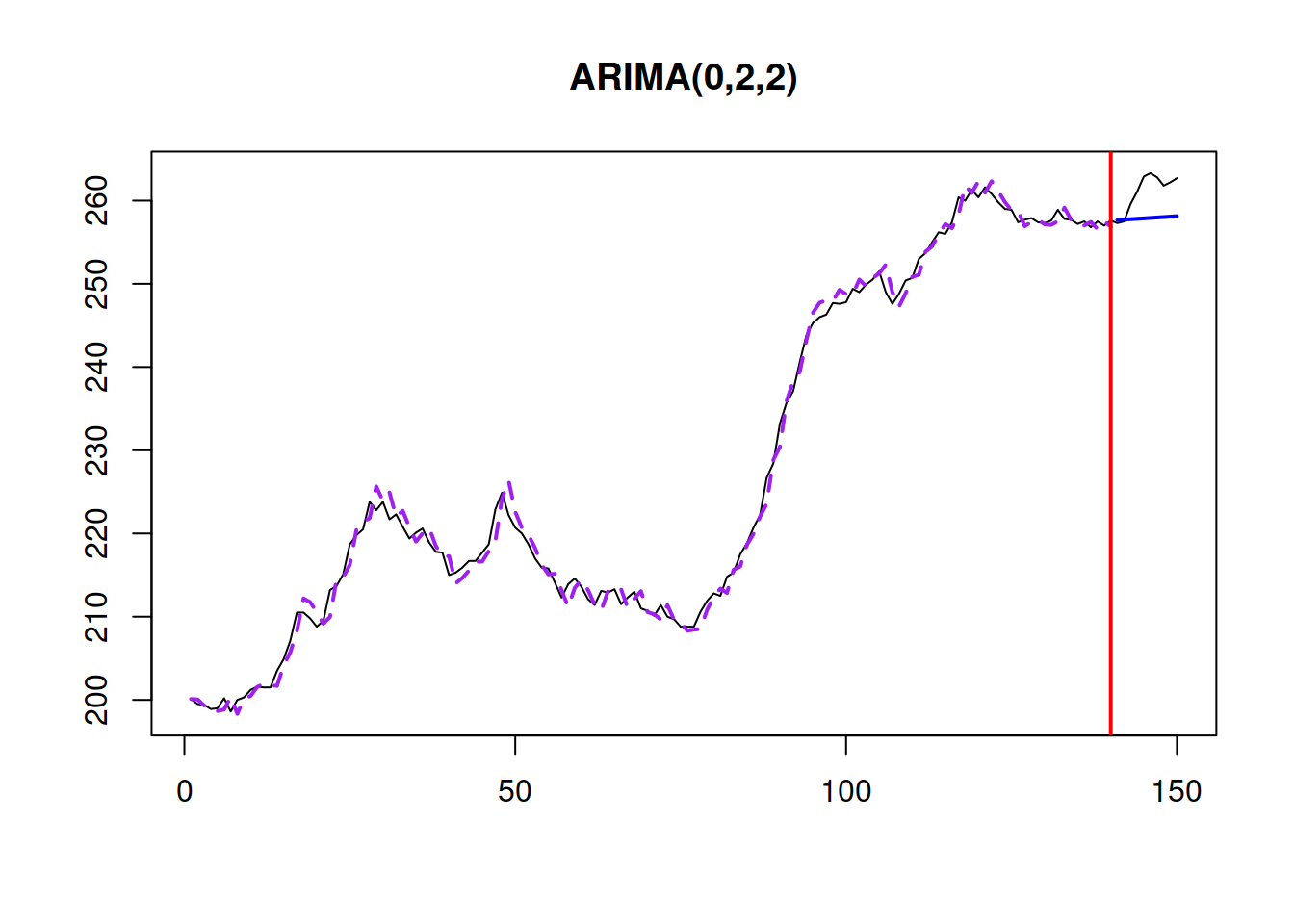
Figure 15.1: Actuals, fitted, and forecast for the Box-Jenkins sales data.
The resulting model will be parsimonious when optimal initials are used. If we want to have a more flexible model, we can use a different initialisation (e.g. backcasting as discussed in Section 11.4), and in some cases, the algorithm will select a model with higher orders of AR, I, and MA.
15.2.1 ETS + ARIMA restrictions
Based on the relation between ARIMA and ETS (see Section 8.4), we do not need to test some of the combinations of models when selecting ARIMA orders. For example, if we already consider ETS(A,N,N), we do not need to check the ARIMA(0,1,1) model. The recommendations for what to skip in different circumstances have been discussed in Section 9.4. Still, there are various ways to construct an ETS + ARIMA model, with different sequences between ETS/ARIMA selection. We suggest starting with ETS components, then moving to the selection of ARIMA orders. This way, we are building upon the robust forecasting model and seeing if it can be improved further by introducing elements that are not there. Note that given the complexity of the task of estimating all parameters for ETS and ARIMA, it is advised to use backcasting (see Section 11.4.1) for the initialisation of such model. Here is an example in R:
adam(AirPassengers, model="PPP",
     orders=list(ar=c(3,3),i=c(2,1),ma=c(3,3),select=TRUE),
     h=10, holdout=TRUE, initial="back")
## Time elapsed: 0.85 seconds
## Model estimated using auto.adam() function: ETS(MMM)+ARIMA(2,0,0)
## With backcasting initialisation
## Distribution assumed in the model: Gamma
## Loss function type: likelihood; Loss function value: 476.779
## Persistence vector g:
## alpha beta gamma
## 0.3697 0.0006 0.2287
##
## ARMA parameters of the model:
## Lag 1
## AR(1) 0.2749
## AR(2) 0.1658
##
## Sample size: 134
## Number of estimated parameters: 6
## Number of degrees of freedom: 128
## Information criteria:
## AIC AICc BIC BICc
## 965.5579 966.2194 982.9450 984.5647
##
## Forecast errors:
## ME: -4.586; MAE: 13.329; RMSE: 18.581
## sCE: -17.331%; Asymmetry: -28.9%; sMAE: 5.037%; sMSE: 0.493%
## MASE: 0.555; RMSSE: 0.596; rMAE: 0.134; rRMSE: 0.15The resulting model is ETS(M,M,M) without any ARIMA elements. This is because having a trend and a seasonal component in ETS will force the automatic mechanism to drop all IMA models and only consider the addition of AR. However, none of the AR seemed to have improved the fit of the model, which is why the pure ETS(M,M,M) was returned.