8.5 Examples of application
8.5.1 Non-seasonal data
Using the time series from the Box-Jenkins textbook (Box and Jenkins, 1976), we fit the ARIMA model to the data but based on our judgment rather than their approach. Just a reminder, here is how the data looks (series BJsales, Figure 8.21):
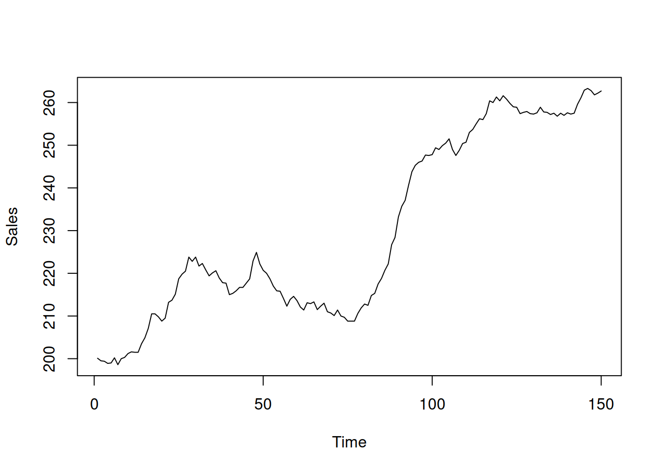
Figure 8.21: Box-Jenkins sales data.
It seems to exhibit the trend in the data, so we can consider ARIMA(1,1,2), ARIMA(0,2,2), and ARIMA(1,1,1) models. We do not consider models with drift in this example, because they would imply the same slope over time for the whole series, which does not seem to be the case here. We use the msarima() function from the smooth package, which is a wrapper for the adam() function:
adamARIMABJ <- vector("list",3)
# ARIMA(1,1,2)
adamARIMABJ[[1]] <- msarima(BJsales, orders=c(1,1,2),
                            h=10, holdout=TRUE)
# ARIMA(0,2,2)
adamARIMABJ[[2]] <- msarima(BJsales, orders=c(0,2,2),
                            h=10, holdout=TRUE)
# ARIMA(1,1,1)
adamARIMABJ[[3]] <- msarima(BJsales, orders=c(1,1,1),
                            h=10, holdout=TRUE)
names(adamARIMABJ) <- c("ARIMA(1,1,2)", "ARIMA(0,2,2)",
                        "ARIMA(1,1,1)")
Comparing information criteria (we will use AICc) of the three models, we can select the most appropriate one:
## ARIMA(1,1,2) ARIMA(0,2,2) ARIMA(1,1,1)
## 488.9598 492.7514 487.0776Remark. Note that this comparison is possible in adam(), ssarima(), and msarima() because the implemented ARIMA is formulated in state space form, sidestepping the issue of the conventional ARIMA (where taking differences reduces the sample size).
Based on this comparison, it looks like the ARIMA(1,1,1) is the most appropriate model (among the three) for the data. Here is how the fit and the forecast from the model looks (Figure 8.22):

Figure 8.22: BJSales series and ARIMA(1,1,1).
Comparing this model with the ETS(A,A,N), we will see a slight difference because the two models are initialised and estimated differently:
## Time elapsed: 0.01 seconds
## Model estimated using adam() function: ETS(AAN)
## With backcasting initialisation
## Distribution assumed in the model: Normal
## Loss function type: likelihood; Loss function value: 243.2882
## Persistence vector g:
##  alpha   beta
## 1.0000 0.2424
##
## Sample size: 140
## Number of estimated parameters: 3
## Number of degrees of freedom: 137
## Information criteria:
##      AIC     AICc      BIC     BICc
## 492.5765 492.7530 501.4014 501.8374
##
## Forecast errors:
## ME: 3.218; MAE: 3.331; RMSE: 3.785
## sCE: 14.129%; Asymmetry: 91.6%; sMAE: 1.462%; sMSE: 0.028%
## MASE: 2.818; RMSSE: 2.483; rMAE: 0.925; rRMSE: 0.921
If we are interested in a more classical Box-Jenkins approach, we can always analyse the residuals of the constructed model and try improving it further. Here is an example of ACF and PACF of the residuals of the ARIMA(1,1,1):
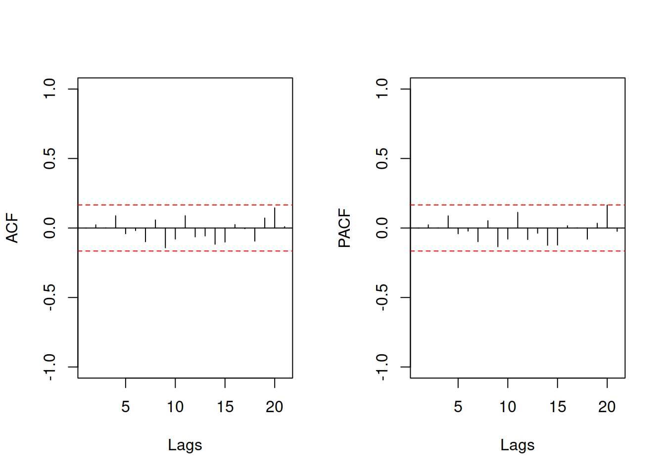
Figure 8.23: ACF and PACF of the ARIMA(1,1,1) model on BJSales data
As we see from the plot in Figure 8.23, all autocorrelation coefficients lie inside the confidence interval, implying that there are no significant AR/MA lags to include in the model.
8.5.2 Seasonal data
Similarly to the previous cases, we use Box-Jenkins AirPassengers data, which exhibits a multiplicative seasonality and a trend. We will model this using SARIMA(0,2,2)(0,1,1)\(_{12}\), SARIMA(0,2,2)(1,1,1)\(_{12}\), and SARIMA(0,2,2)(1,1,0)\(_{12}\) models, which are selected to see what type of seasonal ARIMA is more appropriate to the data:
adamSARIMAAir <- vector("list",3)
# SARIMA(0,2,2)(0,1,1)[12]
adamSARIMAAir[[1]] <- msarima(AirPassengers, lags=c(1,12),
                              orders=list(ar=c(0,0), i=c(2,1),
                                          ma=c(2,1)),
                              h=12, holdout=TRUE)
# SARIMA(0,2,2)(1,1,1)[12]
adamSARIMAAir[[2]] <- msarima(AirPassengers, lags=c(1,12),
                              orders=list(ar=c(0,1), i=c(2,1),
                                          ma=c(2,1)),
                              h=12, holdout=TRUE)
# SARIMA(0,2,2)(1,1,0)[12]
adamSARIMAAir[[3]] <- msarima(AirPassengers, lags=c(1,12),
                              orders=list(ar=c(0,1), i=c(2,1),
                                          ma=c(2,0)),
                              h=12, holdout=TRUE)
names(adamSARIMAAir) <- c("SARIMA(0,2,2)(0,1,1)[12]",
                          "SARIMA(0,2,2)(1,1,1)[12]",
                          "SARIMA(0,2,2)(1,1,0)[12]")
Note that now that we have a seasonal component, we need to provide the SARIMA lags: 1 and \(m=12\) and specify orders differently – as a list with values for AR, I, and MA orders separately. This is done because the SARIMA implemented in msarima() and adam() supports multiple seasonalities (e.g. you can have lags=c(1,24,24*7) if you want). The resulting information criteria of models are:
## SARIMA(0,2,2)(0,1,1)[12] SARIMA(0,2,2)(1,1,1)[12] SARIMA(0,2,2)(1,1,0)[12]
##                 1036.075                 1043.404                 1065.472
It looks like the first model is slightly better than the other two, so we will use it in order to produce forecasts (see Figure 8.24):
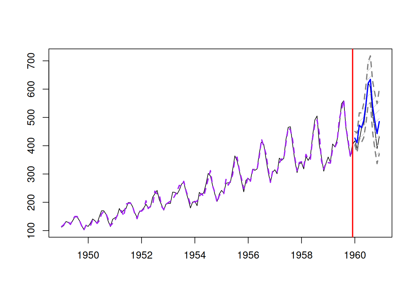
Figure 8.24: Forecast of AirPassengers data from a SARIMA(0,2,2)(0,1,1)\(_{12}\) model.
This model is directly comparable with ETS models, so here is, for example, the AICc value of ETS(M,A,M) on the same data:
## [1] 960.1204It is lower than for the SARIMA model, which means that ETS(M,A,M) is more appropriate for the data in terms of information criteria than SARIMA(0,2,2)(1,1,1)\(_{12}\). We can also investigate if there is a way to improve ETS(M,A,M) by adding some ARMA components (Figure 8.25):
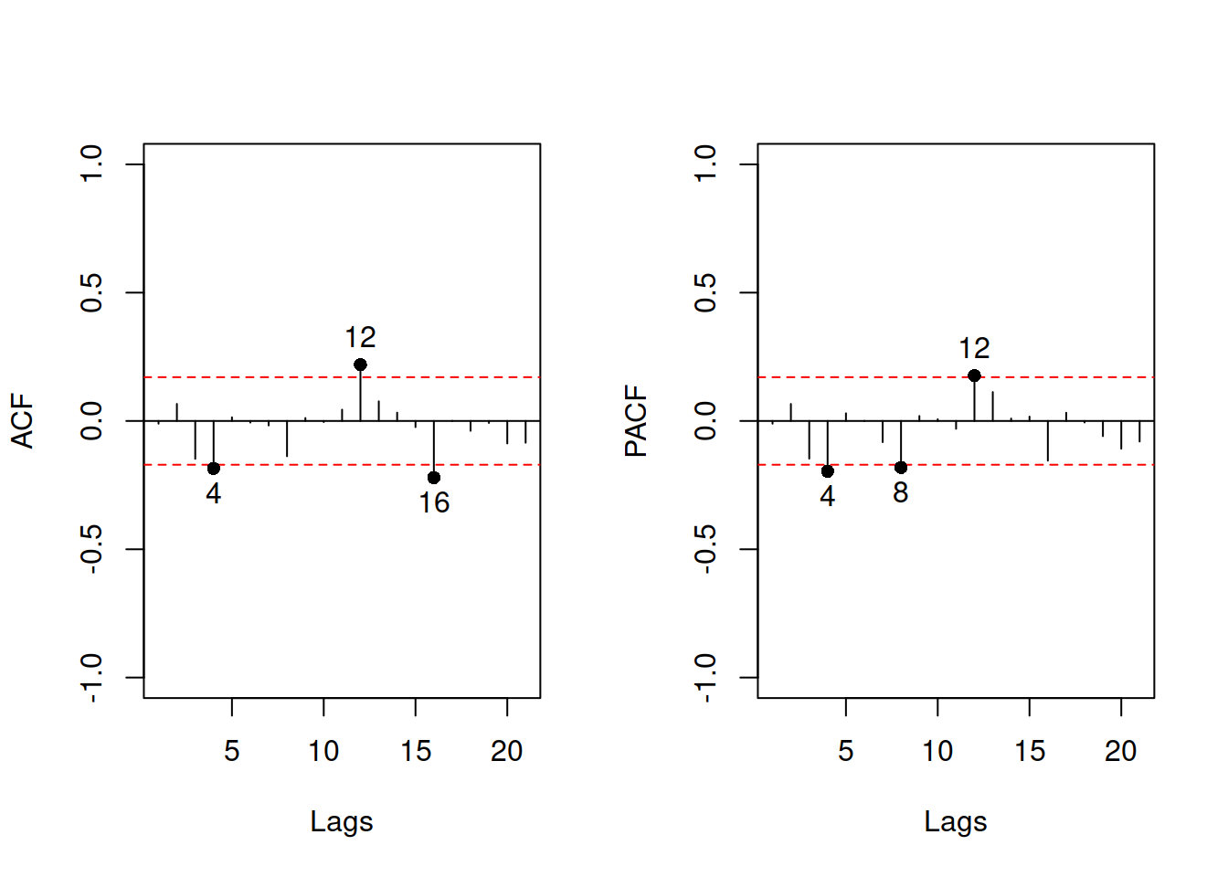
Figure 8.25: ACF and PACF of ETS(M,A,M) on AirPassengers data.
Judging by the plots in Figure 8.25, significant correlation coefficients exist for some lags. Still, it is not clear whether they appear due to randomness or not. Just to check, we will see if adding SARIMA(0,0,0)(0,0,1)\(_{12}\) helps (reduces AICc) in this case:
## [1] 962.9589As we see, the increased complexity does not decrease the AICc (probably because now we need to estimate 13 parameters more than in just ETS(M,A,M)), so we should not add the SARIMA component. We could try adding other SARIMA elements to see if they improve the model, but we do not aim to find the best model here. The interested reader is encouraged to do that as an additional exercise.