4.4 Several examples of ETS and related Exponential Smoothing methods
There are other Exponential Smoothing methods, which include more components, as discussed in Section 3.1. This includes but is not limited to: Holt’s (Holt, 2004, originally proposed in 1957), Holt-Winter’s (Winters, 1960), multiplicative trend (Pegels, 1969), damped trend (originally proposed by Roberts (1982) and then picked up by Gardner and McKenzie (1985)), damped trend Holt-Winters (Gardner and McKenzie, 1989), and damped multiplicative trend (Taylor, 2003a) methods. We will not discuss them here one by one, as we will not use them further in this monograph. Instead, we will focus on the ETS models underlying them.
We already understand that there can be different components in time series and that they can interact either in an additive or a multiplicative way, which gives us the taxonomy discussed in Section 4.1. This section considers several examples of ETS models and their relations to the conventional Exponential Smoothing methods.
4.4.1 ETS(A,A,N)
This is also sometimes known as the local trend model and is formulated similar to ETS(A,N,N), but with addition of the trend equation. It underlies Holt’s method (Ord et al., 1997): \[\begin{equation} \begin{aligned} & y_{t} = l_{t-1} + b_{t-1} + \epsilon_t \\ & l_t = l_{t-1} + b_{t-1} + \alpha \epsilon_t \\ & b_t = b_{t-1} + \beta \epsilon_t \end{aligned} , \tag{4.13} \end{equation}\] where \(\beta\) is the smoothing parameter for the trend component. It has a similar idea as ETS(A,N,N): the states evolve, and the speed of their change depends on the values of \(\alpha\) and \(\beta\). The trend is not deterministic in this model: both the intercept and the slope change over time. The higher the smoothing parameters are, the more uncertain the level and the slope will be, thus, the higher the uncertainty about the future values is.
Here is an example of the data that corresponds to the ETS(A,A,N) model:
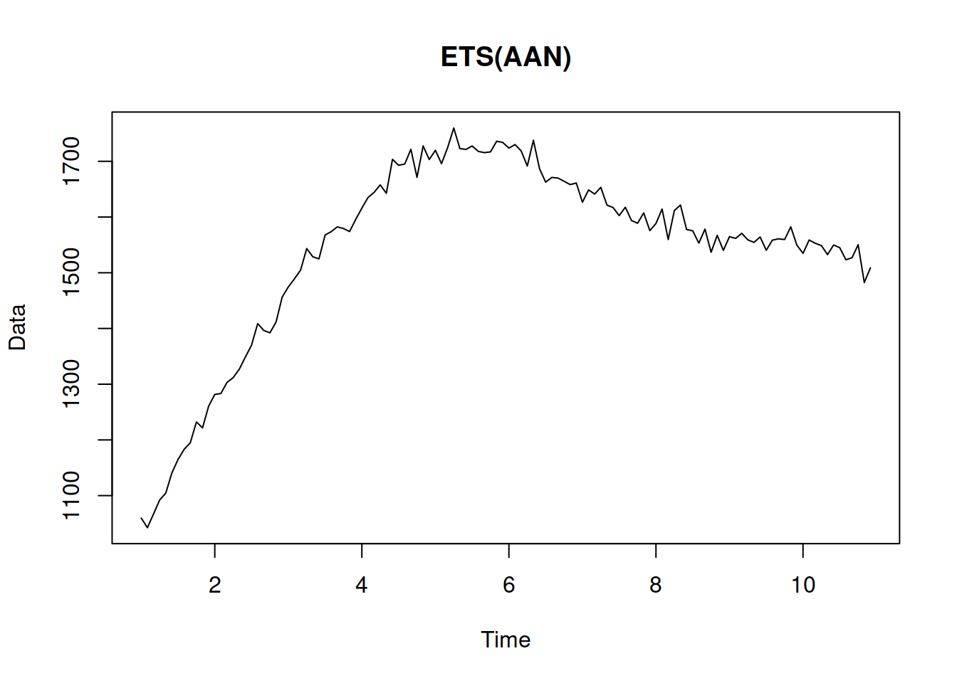
Figure 4.9: Data generated from an ETS(A,A,N) model.
The series in Figure 4.9 demonstrates a trend that changes over time. If we need to produce forecasts for this data, we will capture the dynamics of the trend component via ETS(A,A,N) and then use the last values for the several steps ahead prediction.
The point forecast \(h\) steps ahead from this model is a straight line with a slope \(b_t\) (as shown in Table 4.3 from Section 4.2): \[\begin{equation} \mu_{y,t+h|t} = \hat{y}_{t+h} = l_{t} + h b_t. \tag{4.14} \end{equation}\] This becomes apparent if one takes the conditional expectations E\((l_{t+h}|t)\) and E\((b_{t+h}|t)\) in the second and third equations of (4.13) and then inserts them in the measurement equation. Graphically it will look as shown in Figure 4.10:
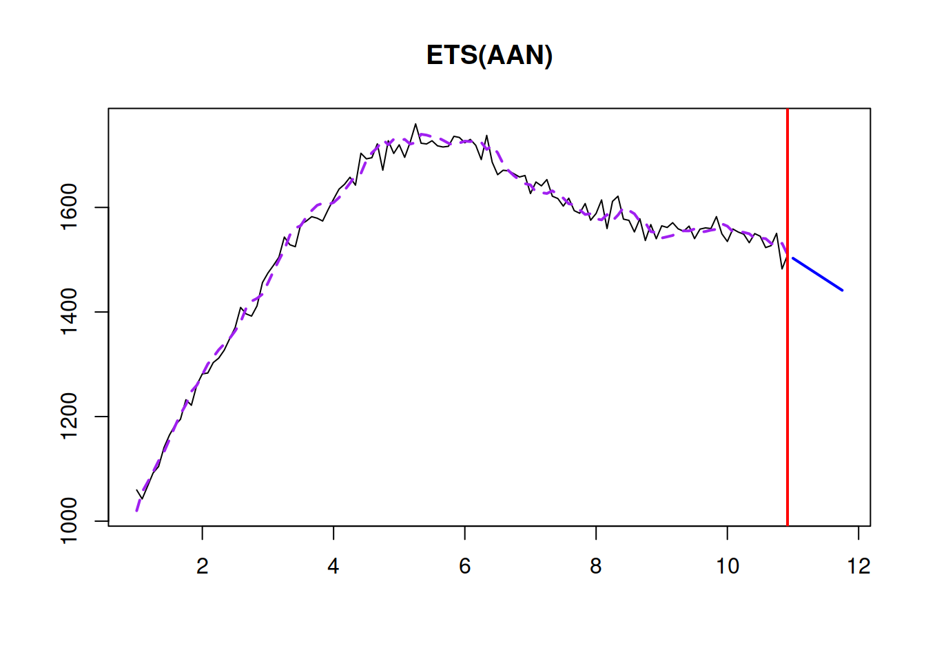
Figure 4.10: ETS(A,A,N) and a point forecast produced from it.
If you want to experiment with the model and see how its parameters influence the fit and forecast, you can use the following R code:
where persistence is the vector of smoothing parameters (first \(\hat\alpha\), then \(\hat\beta\)). By changing their values, we will make the model less/more responsive to the changes in the data.
In a special case, ETS(A,A,N) corresponds to the Random Walk with drift (Subsection 3.3.4), when \(\beta=0\) and \(\alpha=1\): \[\begin{equation*} \begin{aligned} & y_{t} = l_{t-1} + b_{t-1} + \epsilon_t \\ & l_t = l_{t-1} + b_{t-1} + \epsilon_t \\ & b_t = b_{t-1} \end{aligned} , \end{equation*}\] or \[\begin{equation} \begin{aligned} & y_{t} = l_{t-1} + b_{0} + \epsilon_t \\ & l_t = l_{t-1} + b_{0} + \epsilon_t \end{aligned} . \tag{4.15} \end{equation}\] The connection between the two models becomes apparent, when substituting the first equation into the second one in (4.15) to obtain: \[\begin{equation} \begin{aligned} & y_{t} = l_{t-1} + b_{0} + \epsilon_t \\ & l_t = y_{t} \end{aligned} , \end{equation}\] or after inserting the second equation into the first one: \[\begin{equation} y_{t} = y_{t-1} + b_{0} + \epsilon_t . \end{equation}\]
Finally, in another special case, when both \(\alpha\) and \(\beta\) are zero, the model reverts to the Global Trend discussed in Subsection 3.3.5 and becomes: \[\begin{equation*} \begin{aligned} & y_{t} = l_{t-1} + b_{t-1} + \epsilon_t \\ & l_t = l_{t-1} + b_{t-1} \\ & b_t = b_{t-1} \end{aligned} , \end{equation*}\] or \[\begin{equation} \begin{aligned} & y_{t} = l_{t-1} + b_{0} + \epsilon_t \\ & l_t = l_{t-1} + b_{0} \end{aligned} . \tag{4.16} \end{equation}\] The main difference of (4.16) with the Global Trend model (3.13) is that the latter explicitly includes the trend component \(t\) and is formulated in one equation, while the former splits the equation into two parts and has an explicit level component. They both fit the data in the same way and produce the same forecasts when \(a_0 = l_0\) and \(a_1 = b_0\) in the Global Trend model.
Due to its flexibility, the ETS(A,A,N) model is considered as one of the good benchmarks in the case of trended time series.
4.4.2 ETS(A,Ad,N)
This is the model that underlies the damped trend method (Gardner and McKenzie, 1985; Roberts, 1982): \[\begin{equation} \begin{aligned} & y_{t} = l_{t-1} + \phi b_{t-1} + \epsilon_t \\ & l_t = l_{t-1} + \phi b_{t-1} + \alpha \epsilon_t \\ & b_t = \phi b_{t-1} + \beta \epsilon_t \end{aligned} , \tag{4.17} \end{equation}\] where \(\phi\) is the dampening parameter, typically lying between zero and one. If it is equal to zero, the model reduces to ETS(A,N,N), (4.3). If it is equal to one, it becomes equivalent to ETS(A,A,N), (4.13). The dampening parameter slows down the trend, making it non-linear. An example of data that corresponds to ETS(A,Ad,N) is provided in Figure 4.11.
y <- sim.es("AAdN", 120, 1, 12, persistence=c(0.3,0.1),
            initial=c(1000,20), phi=0.95, mean=0, sd=20)
plot(y)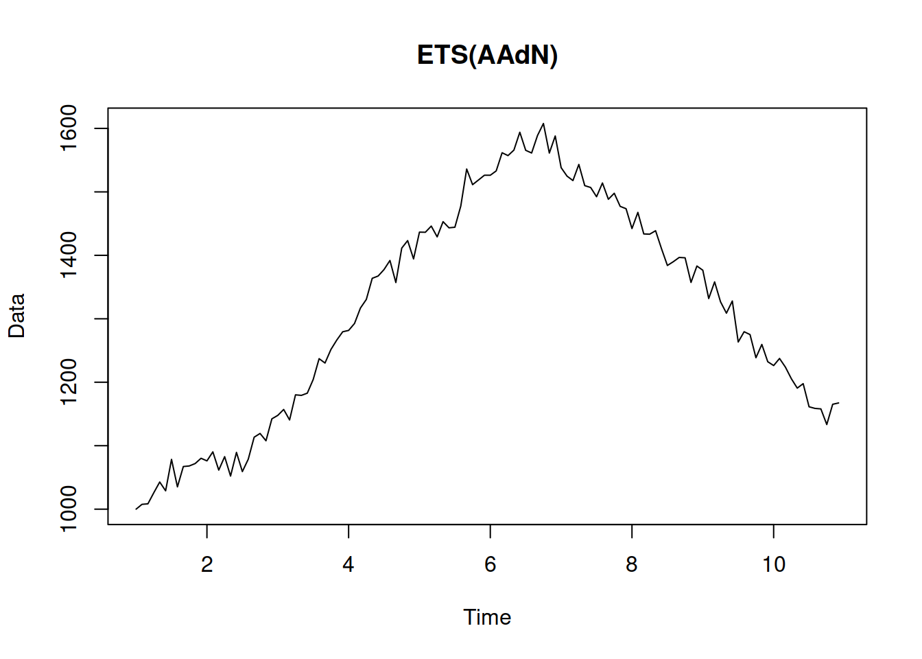
Figure 4.11: An example of ETS(A,Ad,N) data.
Visually it is typically challenging to distinguish ETS(A,A,N) from ETS(A,Ad,N) data. So, some other model selection techniques are recommended (see Section 15.1).
The point forecast from this model is a bit more complicated than the one from ETS(A,A,N) (see Section 4.2): \[\begin{equation} \mu_{y,t+h|t} = \hat{y}_{t+h} = l_{t} + \sum_{j=1}^h \phi^j b_t. \tag{4.18} \end{equation}\] It corresponds to the slowing down trajectory, as shown in Figure 4.12.
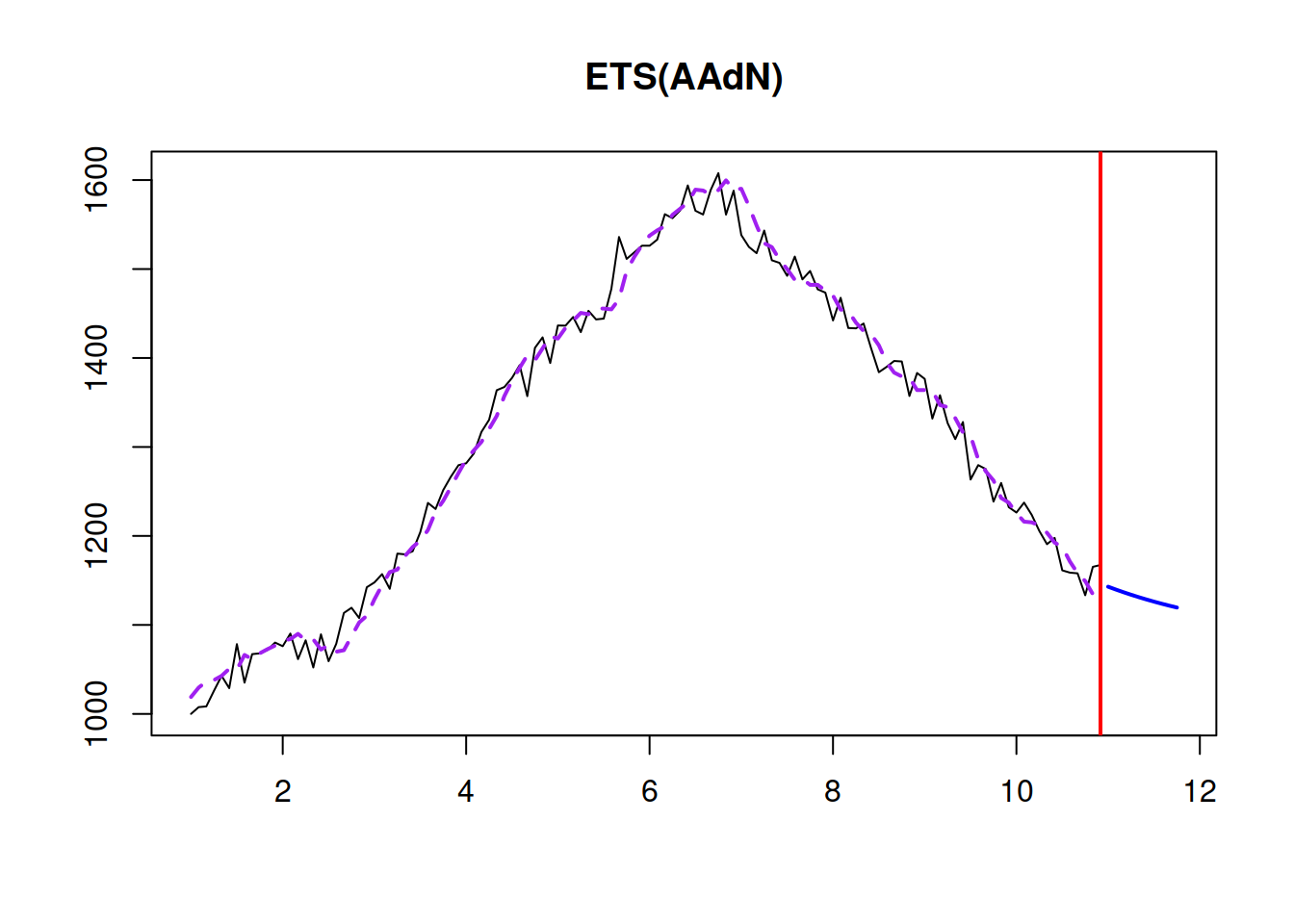
Figure 4.12: A point forecast from ETS(A,Ad,N).
As can be seen in Figure 4.12, the forecast trajectory from the ETS(A,Ad,N) has a slowing down element in it. This is because of the \(\phi=0.95\) in our example.
Finally, to demonstrate the effect of different values of \(\phi\) on model fit and forecasts, we generate a data and then apply several ETS(A,Ad,N) models with \(\phi=0\), \(\phi=0.75\), \(\phi=0.9\), \(\phi=0.95\) and \(\phi=1\) (Figure 4.13).
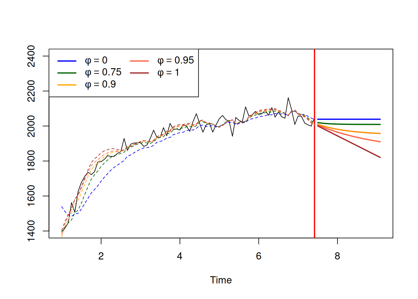
Figure 4.13: ETS(A,Ad,N) applied to some generated data with different values of dampening parameter.
As we see from Figure 4.13, when \(\phi=0\), the model reverts to the ETS(A,N,N) and produces flat trajectory. In the opposite case of \(\phi=1\), it becomes equivalent to the ETS(A,A,N), producing a stright line, going down indefinitely. Finally, with different values of the dampening parameter between zero and one, we see that the trajectories slow down and reach some level. The process is slower the higher the dampening parameter is.
4.4.3 ETS(A,A,M)
Finally, this is an exotic model with additive error and trend, but multiplicative seasonality. It can be considered exotic because of the misalignment of the error and seasonality. Still, we list it here, because it underlies the Holt-Winters method (Winters, 1960): \[\begin{equation} \begin{aligned} & y_{t} = (l_{t-1} + b_{t-1}) s_{t-m} + \epsilon_t \\ & l_t = l_{t-1} + b_{t-1} + \alpha \frac{\epsilon_t}{s_{t-m}} \\ & b_t = b_{t-1} + \beta \frac{\epsilon_t}{s_{t-m}} \\ & s_t = s_{t-m} + \gamma \frac{\epsilon_t}{l_{t-1}+b_{t-1}} \end{aligned} , \tag{4.19} \end{equation}\] where \(s_t\) is the seasonal component and \(\gamma\) is its smoothing parameter. This is one of the potentially unstable models, which due to the mix of components, might produce unreasonable forecasts because the seasonal component might become negative, while it should always be positive. Still, it might work on the strictly positive high-level data. Figure 4.14 shows how the data for this model can look.
y <- sim.es("AAM", 120, 1, 4, persistence=c(0.3,0.05,0.2),
            initial=c(1000,20), initialSeason=c(0.9,1.1,0.8,1.2),
            mean=0, sd=20)
plot(y)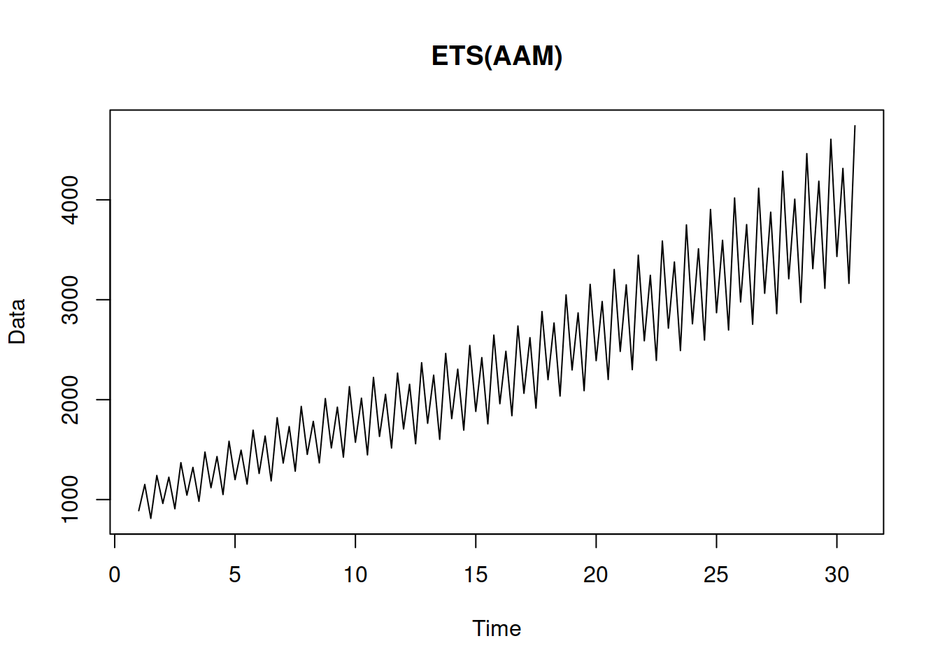
Figure 4.14: An example of ETS(A,A,M) data.
The data in Figure 4.14 exhibits an additive trend with increasing seasonal amplitude, which are the two characteristics of the model.
Finally, the point forecast from this model builds upon ETS(A,A,N), introducing seasonal component: \[\begin{equation} \hat{y}_{t+h} = (l_{t} + h b_t) s_{t+h-m\lceil\frac{h}{m}\rceil}, \tag{4.20} \end{equation}\] where \(\lceil\frac{h}{m}\rceil\) is the rounded up value of the fraction in the brackets, implying that the seasonal index from the previous period is used (e.g. previous January value). The point forecast from this model is shown in Figure 4.15.
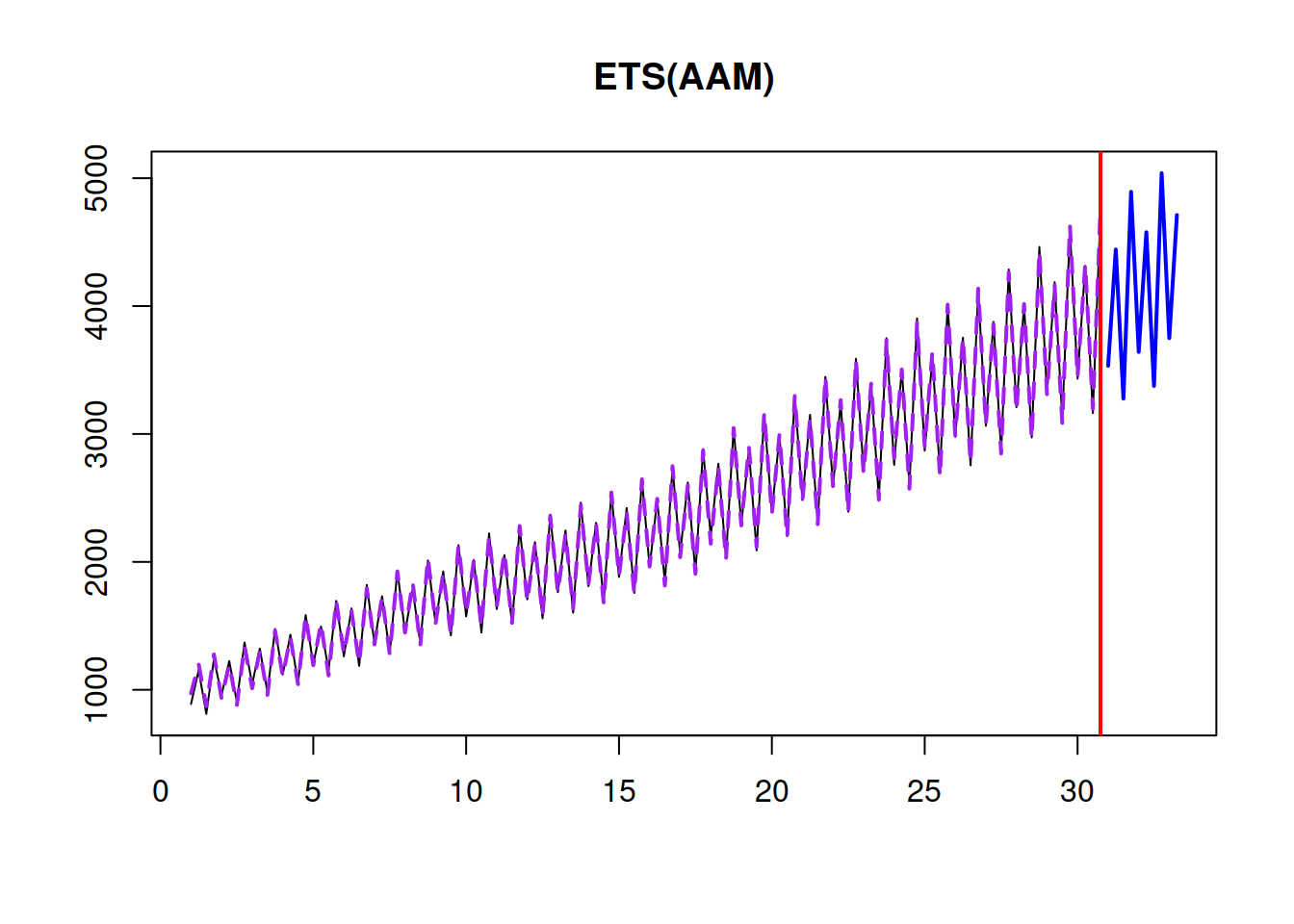
Figure 4.15: A point forecast from ETS(A,A,M).
Remark. The point forecasts produced from this model do not correspond to the conditional expectations. This will be discussed in Section 7.3.
Hyndman et al. (2008) argue that in ETS models, the error term should be aligned with the seasonal component because it is difficult to motivate why the amplitude of seasonality should increase with the increase of level, while the variability of the error term should stay the same. So, they recommend using ETS(M,A,M) instead of ETS(A,A,M) if you deal with positive high-volume data. This is a reasonable recommendation, but keep in mind that both models might break if you deal with the low-volume data and the trend component becomes negative.