13.4 Examples of application
In order to see how ADAM works on intermittent data, we consider the same example from the Section 13.1. We remember that in that example both demand occurrence and demand sizes increase over time, meaning that we can try the model with trend for both parts:
plot(y)
This can be done using adam() function from smooth package, defining the type of occurrence to use. We will try several options and select the one that has the lowest AICc:
adamModelsiETS <- vector("list",4)
adamModelsiETS[[1]] <- adam(y, "MMdN", occurrence="odds-ratio",
                            h=10, holdout=TRUE)
adamModelsiETS[[2]] <- adam(y, "MMdN", occurrence="inverse-odds-ratio",
                            h=10, holdout=TRUE)
adamModelsiETS[[3]] <- adam(y, "MMdN", occurrence="direct",
                            h=10, holdout=TRUE)
adamModelsiETS[[4]] <- adam(y, "MMdN", occurrence="general",
                            h=10, holdout=TRUE)
adamModelsiETSAICcs <- setNames(sapply(adamModelsiETS,AICc),
                                c("odds-ratio","inverse-odds-ratio","direct","general"))
adamModelsiETSAICcs
## odds-ratio inverse-odds-ratio direct general
## 375.9596 369.9136 368.6418 423.5761Based on this, we can see that the model with direct has the lowest AICc. We can see how the model has approximated the data and produced forecasts for the holdout:
i <- which.min(adamModelsiETSAICcs)
plot(adamModelsiETS[[i]],7)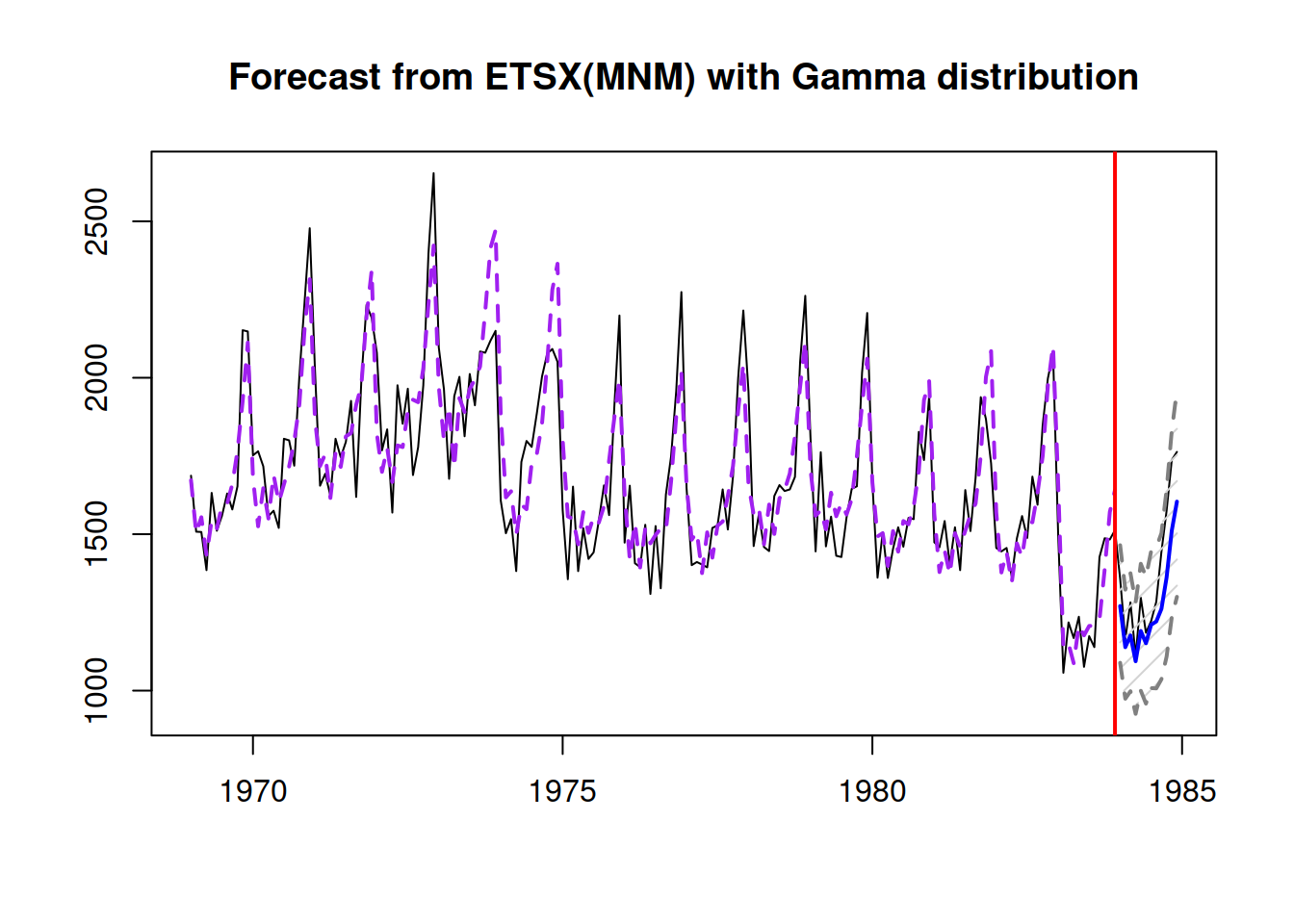
We can explore the demand occurrence part of this model the following way:
adamModelsiETS[[i]]$occurrence## Occurrence state space model estimated: Direct probability
## Underlying ETS model: oETS[D](MMdN)
## Smoothing parameters:
## level trend
## 0 0
## Vector of initials:
## level trend
## 0.2176 1.0206
##
## Error standard deviation: 0.8993
## Sample size: 110
## Number of estimated parameters: 5
## Number of degrees of freedom: 105
## Information criteria:
## AIC AICc BIC BICc
## 95.1229 95.6998 108.6253 109.9812plot(adamModelsiETS[[i]]$occurrence)
Depending on the generated data, there might be issues in the ETS(M,Md,N) model for demand sizes, if the smoothing parameters are large. So, we can try out the ADAM logARIMA(1,1,2) to see how it compares with this model. Given that ARIMA is not yet implemented for the occurrence part of the model, we need to construct it separately and then use in adam():
oETSModel <- oes(y, "MMdN", occurrence=names(adamModelsiETSAICcs)[i],
                 h=10, holdout=TRUE)
adamModeliARIMA <- adam(y, "NNN", occurrence=oETSModel, orders=c(1,1,2),
                        distribution="dlnorm", h=10, holdout=TRUE)
adamModeliARIMA
## Time elapsed: 0.11 seconds
## Model estimated using adam() function: iARIMA(1,1,2)[D]
## Occurrence model type: Direct
## Distribution assumed in the model: Mixture of Bernoulli and Log Normal
## Loss function type: likelihood; Loss function value: 132.806
## ARMA parameters of the model:
## AR:
## phi1[1]
## -0.1047
## MA:
## theta1[1] theta2[1]
## -0.8018 -0.0271
##
## Sample size: 110
## Number of estimated parameters: 6
## Number of degrees of freedom: 104
## Number of provided parameters: 5
## Information criteria:
## AIC AICc BIC BICc
## 362.7349 363.5505 378.9378 380.8545
##
## Forecast errors:
## Asymmetry: 29.471%; sMSE: 193.062%; rRMSE: 1.034; sPIS: -4808.194%; sCE: 493.985%plot(adamModeliARIMA,7)
Comparing the iARIMA model with the previous iETS based on AIC would not be fair, because as soon as the occurrence model is provided to adam(), he does not count the parameters estimated in that part towards the overal number of estimated parameters. In order to make the comparison fair, we need to estimate ADAM iETS in the following way:
adamModelsiETS[[i]] <- adam(y, "MMdN", occurrence=oETSModel,
                            h=10, holdout=TRUE)
adamModelsiETS[[i]]
## Time elapsed: 0.03 seconds
## Model estimated using adam() function: iETS(MMdN)[D]
## Occurrence model type: Direct
## Distribution assumed in the model: Mixture of Bernoulli and Gamma
## Loss function type: likelihood; Loss function value: 130.3517
## Persistence vector g:
## alpha beta
## 0.0548 0.0544
## Damping parameter: 0.7219
## Sample size: 110
## Number of estimated parameters: 6
## Number of degrees of freedom: 104
## Number of provided parameters: 5
## Information criteria:
## AIC AICc BIC BICc
## 357.8262 358.6418 374.0291 375.9458
##
## Forecast errors:
## Asymmetry: 11.937%; sMSE: 172.229%; rRMSE: 0.977; sPIS: -3617.408%; sCE: 285.332%plot(adamModelsiETS[[i]],7)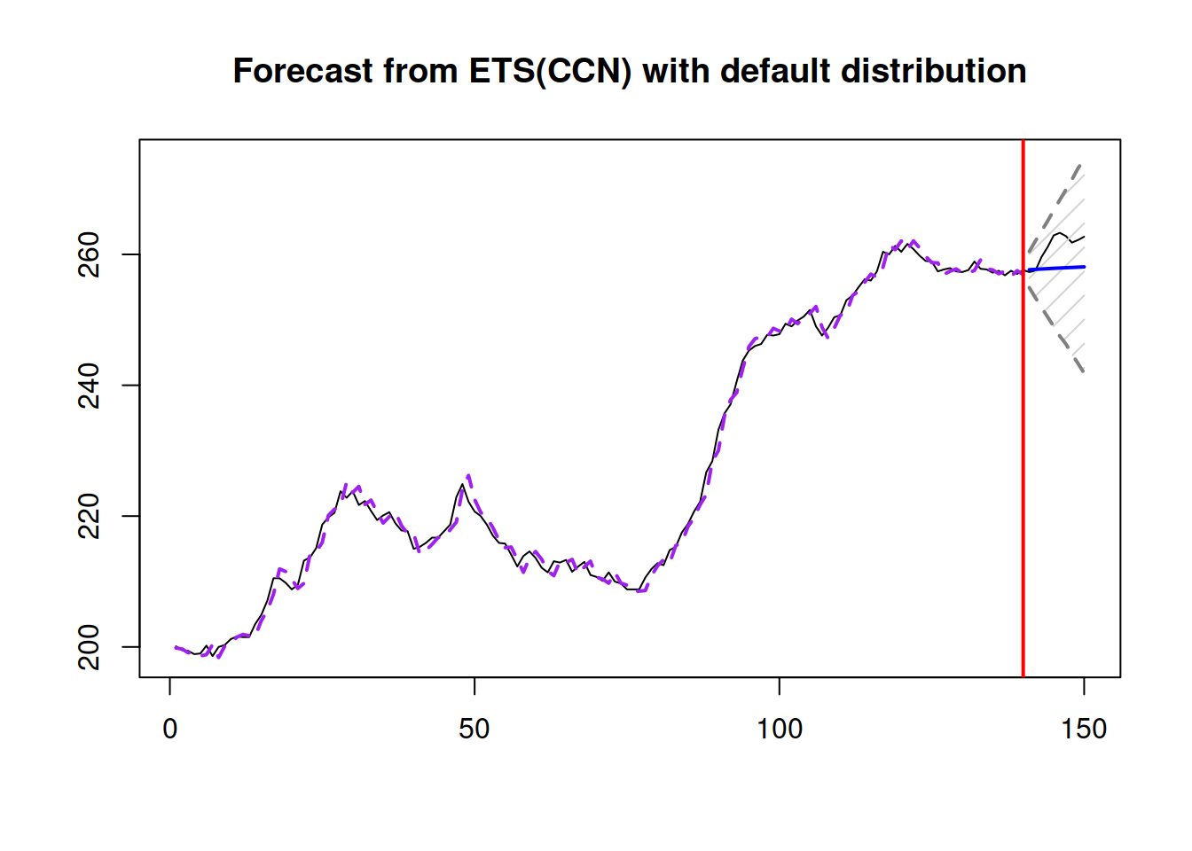
Comparing information criteria, the iETS model is more appropriate for this data. But this might be due to a different distributional assumptions and difficulties estimating ARIMA model. If you want to experiment more with ADAM iARIMA, you might try fine tuning it for the data either by increasing the maxeval or changing the initialisation, for example:
adamModeliARIMA <- adam(y, "NNN", occurrence=oETSModel, orders=c(1,1,2),
                        distribution="dgamma", h=10, holdout=TRUE, initial="back")
adamModeliARIMA
## Time elapsed: 0.1 seconds
## Model estimated using adam() function: iARIMA(1,1,2)[D]
## Occurrence model type: Direct
## Distribution assumed in the model: Mixture of Bernoulli and Gamma
## Loss function type: likelihood; Loss function value: 140.7999
## ARMA parameters of the model:
## AR:
## phi1[1]
## -0.0345
## MA:
## theta1[1] theta2[1]
## -0.8116 0.0487
##
## Sample size: 110
## Number of estimated parameters: 4
## Number of degrees of freedom: 106
## Number of provided parameters: 5
## Information criteria:
## AIC AICc BIC BICc
## 374.7227 375.1037 385.5246 386.4200
##
## Forecast errors:
## Asymmetry: 32.727%; sMSE: 197.377%; rRMSE: 1.046; sPIS: -5019.278%; sCE: 531.51%plot(adamModeliARIMA,7)
Finally, we can produce point and interval forecasts from either of the model via the forecast() method. Here is an example:
adamiETSForecasts <- forecast(adamModelsiETS[[i]],h=10,interval="prediction",nsim=10000)
plot(adamiETSForecasts)
The prediction intervals produced from multiplicative ETS models will typically be simulated, so in order to make them smoother you might need to increase nsim parameter, for example to nsim=100000.