2.5 Hypothesis testing
While we will not need hypothesis testing for ADAM itself, we might face it in some parts of the textbook, so it is worth discussing it briefly.
Hypothesis testing arises naturally from the idea of confidence intervals: instead of constructing the interval and getting the idea about the uncertainty of the parameter, we could check, whether the sample agrees with our expectations or not. For example, we could test, whether the population mean is equal to zero based on our sample. We could either construct a confidence interval for the sample mean and see if zero is included in it (in which case it might indicate that zero is one of the possible values of the population mean), or we could reformulate the problem and compare some calculated value with the theoretical threshold. The latter approach is in the nutshell what hypothesis testing does.
Fundamentally, the hypothesis testing process relies on the ideas of induction and dichotomy: we have a null (H\(_0\)) and alternative (H\(_1\)) hypotheses about the process or a property in the population, and we want to find some evidence to reject the H\(_0\). Rejecting a hypothesis is actually more useful than not rejecting it, because in the former case we know what not to expect from the data, while in the latter we just might not have enough evidence to make any solid conclusion. For example, we could formulate H\(_0\) that all cats are white. Failing to reject this hypothesis based on the data that we have (e.g. a dataset of white cats) does not mean that they are all (in the universe) indeed white, it just means that we have not observed the non-white ones. If we collect enough evidence to reject H\(_0\) (i.e. encountered a black cat), then we can conclude that not all cats are white. This is a more solid conclusion than the one in the previous case. So, if you are interested in a specific outcome, then it makes sense to put this in the alternative hypothesis and see if the data allows to reject the null. For example, if we want to see if the average salary of professors in the UK is higher than £100k per year we would formulate the hypotheses in the following way: \[\begin{equation*} \mathrm{H}_0: \mu \leq 100, \mathrm{H}_1: \mu > 100. \end{equation*}\] Having formulated hypotheses, we can check them, but in order to do that, we need to follow a proper procedure, which can be summarised in the six steps:
- Formulate null and alternative hypotheses (H\(_0\) and H\(_1\)) based on your understanding of the problem;
- Select the significance level \(\alpha\) on which the hypothesis will be tested;
- Select the test appropriate for the formulated hypotheses (1);
- Conduct the test (3) and get the calculated value;
- Compare the value in (4) with the threshold one;
- Make a conclusion based on (5) on the selected level (2).
Note that the order of some elements might change depending on the circumstances, but (2) should always happen before (4), otherwise we might be dealing with so called “p-hacking,” trying to make results look nicer than they really are.
Consider an example, where we want to check, whether the population mean \(\mu\) is equal to zero, based on a sample of 36 observations, where \(\bar{y}=-0.5\) and \(s^2=1\). In this case, we formulate the null and alternative hypotheses: \[\begin{equation*} \mathrm{H}_0: \mu=0, \mathrm{H}_1: \mu \neq 0. \end{equation*}\] We then select the significance level \(\alpha=0.05\) (just as an example) and select the test. Based on the description of the task, this can be either a t-test, or a z-test, depending on whether the variance of the variable is known or not. Usually it is not, so we tend to use t-test. We then conduct the test using the formula: \[\begin{equation} t = \frac{\bar{y} - \mu}{s_{\bar{y}}} = \frac{-0.5 - 0}{\frac{1}{\sqrt{36}}} = -3 . \tag{2.6} \end{equation}\] After that we get the critical value of t with \(df=36-1=35\) degrees of freedom and significance level \(\alpha/2=0.025\), which is approximately equal to -2.03. We compare this value with the (2.6) by absolute and reject H\(_0\) if the calculated value is higher than the critical one. In our case it is, so it appears that we have enough evidence to say that the population mean is not equal to 0, on the 5% significance level.
Visually, the whole process of hypothesis testing explained above can be represented in the following way:
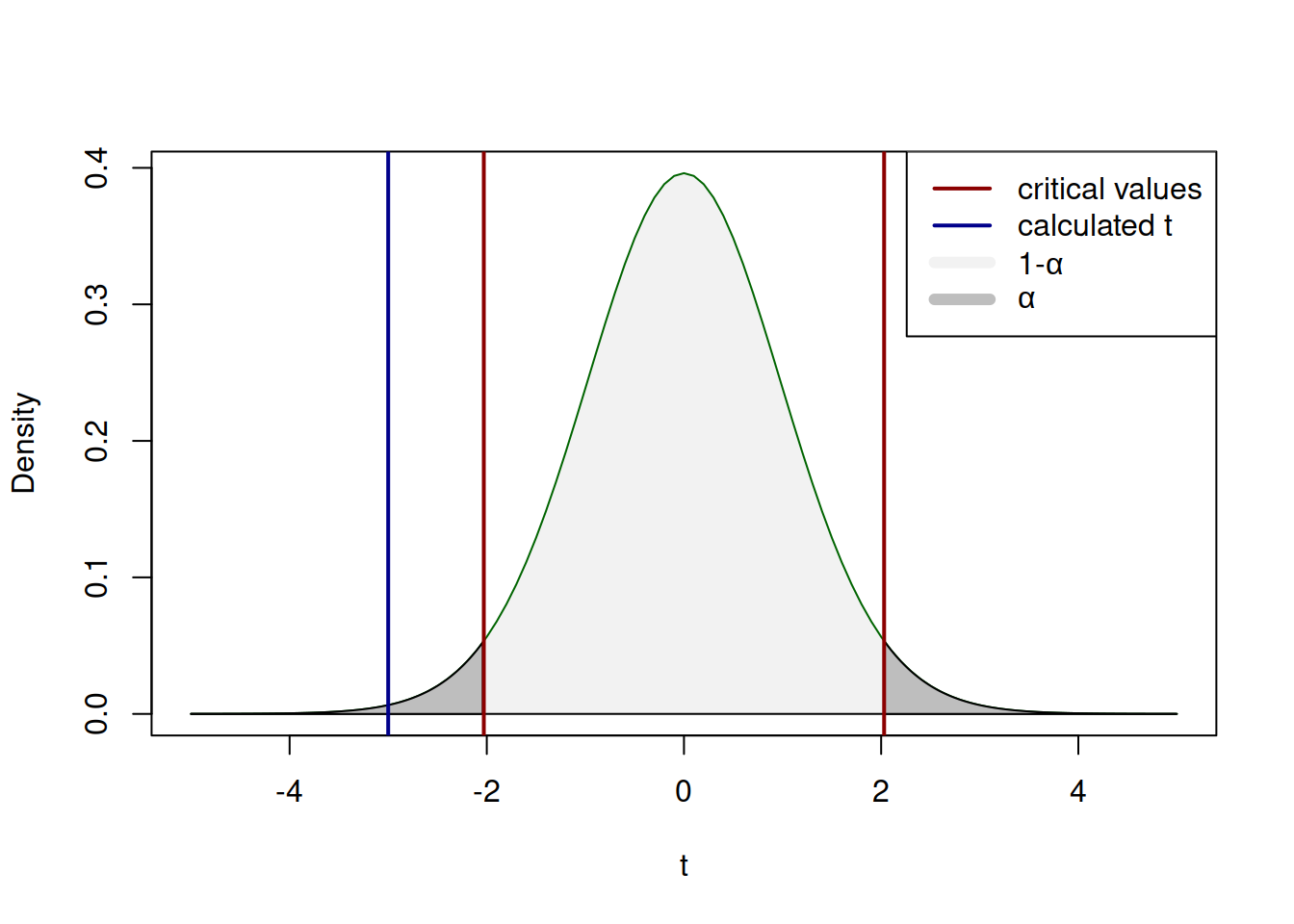
Figure 2.26: The process of hypothesis testing with t value.
If the blue line on Figure 2.26 would lie inside the red bounds (i.e. the calculated value is less than the critical value by absolute), then we would fail to reject H\(_0\). But in our example it is outside the bounds, so we have enough evidence to conclude that the population mean is not equal to zero on 5% significance level. Notice, how similar the mechanisms of confidence interval construction and hypothesis testing are. This is because they are one and the same thing, presented differently. In fact, we could test the same hypothesis by constructing the 95% confidence interval using (2.4) and checking, whether the interval covers the \(\mu=0\): \[\begin{equation*} \begin{aligned} & \mu \in \left(-0.50 -2.03 \frac{1}{\sqrt{36}}, -0.50 + 2.03 \frac{1}{\sqrt{36}} \right), \\ & \mu \in (-0.84, -0.16). \end{aligned} \end{equation*}\] In our case it does not, so we conclude that we reject H\(_0\) on 5% significance level. This can be roughly represented by the graph on Figure 2.27:
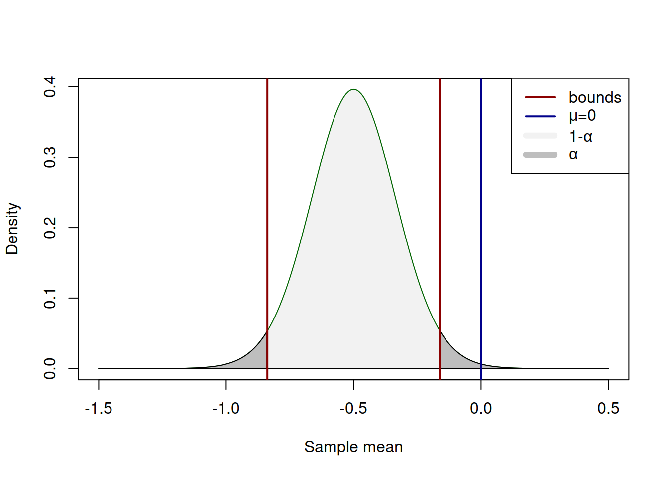
Figure 2.27: The process of hypothesis testing with t value.
Note that the positioning of the blue line has changed in the case of confidence interval, which happens because of the transition from (2.6) to (2.4). The idea and the message, however, stay the same: if the value is not inside the light grey area, then we reject H\(_0\) on the selected significance level.
Also note that we never say that we accept H\(_0\), because this is not what we do in hypothesis testing: if the value would lie inside the interval, then this would only mean that our sample shows that the tested value is covered by the region - the true value can be any of the numbers between the bounds.
Finally, there is a third way to test the hypothesis. We could calculate how much surface is left in the tails with the cut off of the assumed distribution by the blue line on Figure 2.26 (calculated value). In R this can be done using the pt() function:
pt(-3, 36-1)## [1] 0.002474416Given that we had the inequality in the alternative hypothesis, we need to consider both tails, multiplying the value by 2 to get approximately 0.0049. This is the significance level, for which the switch from “reject” to “do not reject” happens. We could compare this value with the pre-selected significance level directly, rejecting H\(_0\) if it is lower than \(\alpha\). This value is called “p-value” and simplifies the hypothesis testing, because we do not need to look at critical values or construct the confidence interval. There are different definitions of what it is, I personally find the following easier to comprehend: p-value is the smallest significance level at which a null hypothesis can be rejected.
Despite this simplification, we still need to follow the procedure and select \(\alpha\) before conducting the test! We should not change the significance level after observing the p-values, otherwise we might end up bending reality for our needs. Also note that if in one case p-value is 0.2, while in the other it is 0.3, it does not mean that the the first case is more significant than the second! P-values are not comparable with each other and they do not tell you about the size of significance. This is still a binary process: we either reject, or fail to reject H\(_0\), depending on whether p-value is smaller or greater than the selected significance level.
While p-value is a comfortable instrument, I personally prefer using confidence intervals, because they show the uncertainty clearer and are less confusing. Consider the following cases to see what I mean:
- We reject H\(_0\) because t-value is -3, which is smaller than the critical value of -2.03 (or equivalently the absolute of t-value is 3, while the critical is 2.03);
- We reject H\(_0\) because p-value is 0.0049, which is smaller than the significance level \(\alpha=0.05\);
- The confidence interval for the mean is \(\mu \in (-0.84, -0.16)\). It does not include zero, so we reject \(\mathrm{H}_0\).
In case of (3), we not only get the same message as in (1) and (2), but we also see how far the bound is from the tested value. In addition, in the situation, when we fail to reject H\(_0\), the approach (3) gives more appropriate information. Consider the case, when we test, whether \(\mu=-0.6\) in the example above. We then have the following three approaches to the problem:
- We fail to reject H\(_0\) because t-value is 0.245, which is smaller than the critical value of 2.03;
- We fail to reject H\(_0\) because p-value is 0.808, which is greater than the significance level \(\alpha=0.05\);
- The confidence interval for the mean is \(\mu \in (-0.84, -0.16)\). It includes -0.6, so we fail to reject H\(_0\). This does not mean that the true mean is indeed equal to -0.6, but it means that the region will cover this number in 95% of cases if we do resampling many times.
In my opinion, the third approach is more informative and saves from making wrong conclusions about the tested hypothesis, making you work a bit more (you cannot change the confidence level on the fly, you would need to reconstruct the interval). Having said that, either of the three is fine, as long as you understand what they really imply.
Furthermore, if you do hypothesis testing and use p-values, it is worth mentioning the statement of American Statistical Association about p-values (Wasserstein and Lazar, 2016). Among the different aspects discussed in this statement, there is a list of principles related to p-values, which I cite below:
- P-values can indicate how incompatible the data are with a specified statistical model;
- P-values do not measure:
- the probability that the studied hypothesis is true,
- or the probability that the data were produced by random chance alone;
- Scientific conclusions and business or policy decisions should not be based only on whether a p-value passes a specific threshold;
- Proper inference requires full reporting and transparency;
- A p-value, or statistical significance, does not measure:
- the size of an effect
- or the importance of a result;
- By itself, a p-value does not provide a good measure of evidence regarding a model or hypothesis.
The statement provides more details about that, but summarising, whatever hypothesis you test and however you test it, you should have apriori understanding of the problem. Diving in the data and trying to see what floats (i.e. which of the p-values is higher than \(\alpha\)) is not a good idea (Wasserstein and Lazar, 2016). Follow the proper procedure if you want to test the hypothesis.
Finally, the hypothesis testing mechanism has been criticised by many scientists over the years. For example, Cohen (1994) discussed issues with the procedure, making several important points, some of which are outlined above. He also points out at the fundamental problem with hypothesis testing, which is typically neglected by proponents of the procedure: in practice, null hypothesis is always wrong. In reality, it is not possible for a value to be equal, for example, to zero. Even an unimportant effect of one variable on another would be close to zero, but not equal to it. This means that with the increase of the sample size, H\(_0\) will inevitably be rejected. Furthermore, our mind operates with binary constructs: true / not true - while the hypothesis testing works in the dichotomy “I know / I don’t know,” with the latter appearing when there is not enough evidence to reject H\(_0\). Summarising all of this, in my opinion, it makes sense to move away from hypothesis testing if possible and switch to other instruments for uncertainty measurement, such as confidence intervals.
2.5.1 Common mistakes related to hypothesis testing
Over the years of teaching statistics, I have seen many different mistakes, related to hypothesis testing. No wonder, this is a difficult topic to grasp. Here, I have decided to summarise several typical erroneous statements, providing explanations why they are wrong. They partially duplicate the 6 principles from ASA discussed above, but they are formulated slightly differently.
- “Calculated value is lower than the critical one, so the null hypothesis is true.”
- This is wrong on so many level, that I do not even know where to start. We can never know if the hypothesis is true or wrong. All the evidence might point towards the H\(_0\) being correct, but it still can be wrong and at some point in future one observation might reject it. The classical example is the “Black swan in Australia.” Up until the discover of Australia, the Europeans thought that there only exist white swans. This was supported by all the observations they had. Wise people would say that “We fail to reject H\(_0\) that all swans are white.” Uneducated people would be tempted to say that " H\(_0\): All swans are white" is true. After discovering Australia in 1606, Europeans have collected evidence of existence of black swans, thus rejecting H\(_0\) and showing that “not all swans are white,” which implies that actually the alternative hypothesis is true. This is the essence of scientific method: we always try rejecting H\(_0\), collecting some evidence. If we fail to reject it, it might just mean that we have not collected enough evidence or have not modelled it correctly.
- “Calculated value is lower than the critical one, so we accept the null hypothesis.”
- We never accept null hypothesis. Even if your house is on fire or there is a tsunami coming, you should not “accept H\(_0\).” This is a fundamental statistical principle. We collect evidence to reject the null hypothesis. If we do not have enough evidence, then we just fail to reject it, but we can never accept it, because failing to reject just means that we need to collect more data. As mentioned earlier, we focus on rejecting hypothesis, because this at least tells us, what the phenomenon is not (e.g. that not all swans are white).
- “The parameter in the model is significant, so we can conclude that…”
- You cannot conclude if something is significant or not without specifying the significance level. Things are only significant if they pass specific test on a specified level \(\alpha\). The correct sentence would be “The parameter in the model is significant on 3%, so we can conclude that…,” where 3% is the selected significance level \(\alpha\).
- “The parameter in the model is significant because p-value<0.0000”
- Indeed, some statistical software will tell you that
p-value<0.0000, but this just says that the value is very small and cannot be printed. Even if it is that small, you need to state your significance level and compare it with the p-value. You might wonder, “why bother if it is that low?” Well, if you change the sample size or change model specification, your p-value will change as well, and in some cases it might all of a sudden become higher than your significance level. So, you always need to keep it in mind and make conclusions based on the significance level, not just based on what software tells you.
- “The parameter is not significant, so we remove the variable from the model.”
- This is one of the worst motivations for removing variables that there is (statistical blasphemy!). There are thousands of reasons, why you might get p-value greater than your significance level (assumptions do not hold, sample is too small, the test is too weak, the true value is small etc) and only one of them is that the explanatory variable does not impact the response variable and thus you fail to reject H\(_0\). Are you sure that you face exactly this one special case? If yes, then you already have some other (better) reasons to remove the variable. This means that you should not make decisions just based on the results of a statistical test. You always need to have some fundamental reason to include or remove variables in the model. Hypothesis testing just gives you additional information that can be helpful for decision making.
- “The parameter in the new model is more significant than in the old one.”
- There is no such thing as “more significant” or “less significant.” Significance is binary and depends on the selected level. The only thing you can conclude is whether the parameter is significant on the chosen level \(\alpha\) or not.
- “The p-value of one variables is higher than the p-value of another, so….”
- p-values are not comparable between variables. They only show on what level the hypothesis is rejected and only work together with the chosen significance level. (6) is similar to this mistake.
Remember that the p-value itself is random and will change if you change the sample size or the model specification. Always keep this in mind, when conducting statistical tests. All these mistakes typically arise because of the misuse of p-values and hypothesis testing mechanism. This is one of the reasons, why I prefer confidence intervals, when possible (as discussed above).
Finally, a related question to all of this, is how to select the significance level. Dave Worthington, a colleague of mine and a Statistics mentor at Lancaster University, has proposed an interesting motivation for that. If you do not have a level, driven by the problem (e.g. we need to satisfy 99% of demand, thus the significance level is 1%), then select the one for your life time. In how many cases in your life would you be ready to make a mistake? Would it be 5%? 3%? 1%? Select something and stick with it. Then over the years you will know that you have made the selected proportion of mistakes, when conducting different statistical test in variaous circumstances.